Paper Outline

Working title: Forcing history shapes the directional state of tropical-cyclone wave fields

Abstract

Tropical cyclone wave fields evolve under rapidly changing wind speed and direction, such that the observed sea state may reflect not only instantaneous forcing but also the recent history of the coupled wind–wave system.

Here, we use directional wave spectra from autonomous surface buoys deployed in four tropical cyclones to examine how spectral structure evolves through these strongly nonstationary conditions.

We characterize the wave field using complementary measures of spectral scale, surface slope, high-frequency energy, and directional organization, including peak frequency (f_p), mean square slope (MSS), directional spreading, and the directional offset between the spectral peak and high-frequency wave field.

Dimensionality reduction reveals a structured, low-dimensional continuum in which spectral properties vary smoothly rather than forming isolated populations. Density-based clustering further tests this structure: HDBSCAN can partition locally dense regions of the observations, but no parameterization simultaneously produces high coverage and well-separated clusters, and categorical solutions are sensitive to feature definition. Instead, when cluster membership is examined independently in time, clusters preferentially occur sequentially across individual storms and buoys, indicating that they partition portions of storm evolution rather than representing persistent wave-state classes.

Wind-forcing models provide a physical interpretation for this organization. Bulk energetic properties are comparatively well described by instantaneous forcing, whereas directional and multiscale spectral properties retain additional information about prior forcing; models incorporating wind history produce their largest improvements for directional quantities and relationships between spectral frequency bands.

Together, these results show that tropical cyclone wave fields are not uniquely determined by the instantaneous local wind, but instead evolve along path-dependent trajectories through a continuous spectral state space.

The spectrum therefore retains information about the forcing history of the storm, with memory expressed most strongly in directional and cross-frequency organization. This challenges an equilibrium view in which the local sea state can be specified from instantaneous wind forcing alone and suggests that rapidly evolving tropical cyclone wave fields require a state description that includes both present forcing and prior evolution.

Because the spectral properties that retain this memory include short-wave slope and directional structure, the results further imply that the wave-mediated air–sea boundary condition itself may be history dependent.

1. INTRODUCTION

1.1 Tropical-cyclone wave fields as evolving systems

(WRITE: ~150–200 words)

Establish that TC wave fields are spatially heterogeneous and rapidly evolving because wind speed and direction change on scales comparable to wave growth, propagation, and adjustment. Therefore, a spectrum observed at one point is not necessarily an equilibrium response to instantaneous local wind.

(ADD: Literature on TC wave-field heterogeneity, nonstationarity, wave growth/adjustment timescales, and propagation)

1.2 Bulk descriptions do not uniquely define wave state

(WRITE: ~150 words)

Introduce the distinction between energetic/spectral-scale quantities and directional organization. Motivate that spectra with similar Hs and fp can differ in directional distribution and high-frequency structure.

(ADD: Literature on directional complexity, mixed seas, and TC spectral structure) (ESTABLISH FROM RESULTS, NOT AS AN ASSUMPTION: Directional spreading is an independent degree of freedom)

1.3 The forcing-history problem

(WRITE: ~150–200 words)

Establish that the present wave field reflects contemporary forcing plus prior evolution. Historical dependence can arise from finite growth/decay timescales, propagation, changing wind direction, nonlinear spectral interactions, and spectral adjustment. Emphasize that TC winds are autocorrelated. The relevant question is whether prior forcing contains information about present wave state that is not already represented by instantaneous forcing.

(ADD: Literature on wave-field memory, turning winds, non-equilibrium response, and spectral adjustment)

1.4 Objectives

(WRITE)

State:

1. Do observed TC wave fields occupy discrete regimes or a continuous low-dimensional state space?
2. Is that state-space structure shared across storms?
3. Does forcing history provide predictive information beyond instantaneous forcing?

End with a brief result preview: energetic and directional properties constitute partially independent dimensions of a shared continuous state space, and historical forcing provides disproportionately large additional predictive information for directional properties.

2. DATA AND METHODS

2.1 Observational dataset and TC-relative forcing

(INSERT / WRITE EXISTING METHODS)

Include storms, Spotter observations, sampling, spectral products, QC, TC tracks, atmospheric forcing, collocation, storm-relative coordinates, radius, and azimuth.

(MAKE FIGURE 1: Dataset overview)

Show storm tracks and buoy observations/trajectories for all storms. Color by storm or local wind speed. Keep this figure descriptive rather than analytical.

2.2 Definition of wave state

(INSERT / WRITE EXISTING DEFINITIONS)

Original state-space vector: (fp, MSS, directional spread, high-frequency tail exponent)

Expanded GAM responses: Hs, MSS, fp, Rhf, HFDS, FPDS, PHFO

Explain which aspect of wave state each metric represents.

(ADD: Exact equations for FPDS, HFDS, PHFO, Rhf, MSS, and tail exponent) (CHECK: Use one consistent directional-spreading definition) (ADD: High-frequency band definitions and rationale)

2.3 Identification of wave-state structure

2.3.1 HDBSCAN

(WRITE METHODS BRIEFLY) State that HDBSCAN tests whether the standardized feature space naturally partitions into density-separated states. (ADD ANALYSIS: Document hyperparameter sensitivity) Report tested parameter ranges, cluster number, noise fraction, and persistence/stability. (MAKE SUPPLEMENTARY FIGURE S1: HDBSCAN sensitivity) Show cluster number/noise fraction/persistence across parameter choices.

2.3.2 PCA

(WRITE METHODS: ~1–2 paragraphs) Include z-score standardization and explain PCA as the dominant linear covariance structure of the four wave-state variables. (ADD: Exact explained-variance percentages for retained PCs) (REMOVE FROM MAIN PAPER: Full covariance/eigendecomposition tutorial)

2.3.3 Isomap

(WRITE METHODS: ~1 paragraph) Explain that PCA supplies interpretable linear axes and Isomap represents nonlinear intrinsic geometry suggested by curved trajectories. Include input variables, k-nearest-neighbor graph, selected k, embedding dimensionality, and selection criterion. (ADD ANALYSIS: Test sensitivity to k) (MAKE SUPPLEMENTARY FIGURE S2: Isomap neighborhood-size sensitivity)

2.3.4 Wave-state trajectories

(INSERT EXISTING FOUR-PARAMETER TRAJECTORY METHOD) Distinguish the global state-space geometry from individual storm/buoy trajectories projected through it. (ADD: Exact four parameters, fitting procedure, and reconstruction/error metric)

2.4 GAM representation of instantaneous forcing

(INSERT EXISTING GAM METHODS)

Include transformations, predictors, GAM form, smoothing basis/k, interactions, LOSO procedure, and explained-deviance definition.

(EMPHASIZE: Reported predictive skill is held-out-storm LOSO skill)

(ADD: Null/reference model and treatment of directional predictors)

2.5 Historical forcing representations

(INSERT EXISTING HISTORY METHODS)

Define instantaneous (I), cumulative (C), Gaussian-localized (G), parallel/perpendicular components, and tested lag/history timescale T.

Explain the physical hypothesis represented by each family.

(MAKE SUPPLEMENTARY TABLE S1: Complete forcing-history model grid)

(MAKE SUPPLEMENTARY FIGURE S3: Full lag/timescale/model-selection curves)

3. RESULTS

3.1 TC wave states form a continuous, low-dimensional space

1. Question: Do the observed wave spectra organize into distinct, recurring wave states?
   • Apply HDBSCAN to the spectral descriptors f_p, MSS, FPDS, and PHFO.
   • These variables span bulk spectral scale, short-wave energy, and directional structure, so discrete physical regimes should appear as persistent density-separated groups if they exist.
2. First result: HDBSCAN can identify clusters, but it cannot identify a robust categorical partition.
   • Across parameter choices, there is a fundamental tradeoff between assigning observations to clusters and obtaining well-separated clusters.
   • Permissive solutions classify more observations but have poor DBCV; more restrictive solutions improve apparent separation only by labeling most observations as noise. 
   • Thus, there is no density scale at which the observations naturally resolve into a small set of clean spectral states.
3. The apparent clusters substantially overlap in spectral space.
   • Representative solutions occupy overlapping regions of PCA space rather than isolated clouds.
   • Individual distributions of f_p, MSS, FPDS, and PHFO also overlap substantially between clusters. 
   • HDBSCAN is therefore partitioning structure within a continuous distribution rather than discovering sharply separated spectral populations.
4. The categorical answer is also sensitive to how the wave state is defined.
   • Removing directional variables or adding R_{hf} can substantially change the number of recovered clusters and agreement between solutions. 
   • If the clusters represented fundamental physical regimes, their identities should be substantially more invariant to reasonable changes in feature definition.
   • Conclusion from Figure 1: HDBSCAN does not support a robust categorical wave-state taxonomy. 

Figure 1. DBCV = density based clustering validation (measures whether each cluster is internally density-connected while being density-separated from neighboring clusters) (DBCV<0 : within-cluster density gaps are comparable to or worse than the gaps between clusters — poor evidence for genuine density-separated groups) Panel A) No density setting gives both coverage and separation. ARI = adjusted rand index (asks : given the same observations clustered in two different ways, how similar are the assignments?)

5. But the failure of a categorical taxonomy does not mean the clusters are meaningless.
   • This motivates a different question: what structure is HDBSCAN actually partitioning?
   • Examine cluster membership in time, while still deriving the clusters exclusively from spectral variables—time and location are not supplied to HDBSCAN.
6. Second result: cluster membership is strongly organized by storm evolution.
   • Within each storm, cluster colors generally progress from early-time to late-time clusters rather than appearing randomly throughout the observational period.
   • Individual buoys tend to move through similar sequences of spectral clusters as the storm evolves.
   • This temporal organization emerges independently even though time was absent from the clustering feature space.
7. Ian provides a particularly clear example of sequential evolution.
   • Early observations preferentially occupy the blue clusters, followed by intermediate purple states and then darker late-time clusters.
   • Similar transitions occur across multiple buoys at approximately comparable stages of the storm.
   • The clusters therefore behave more like successive portions of an evolving spectral trajectory than independent wave-state classes.
8. Idalia shows the same behavior with finer subdivision.
   • Eight recovered clusters partition the observational sequence into a relatively ordered progression from early to late states.
   • Different buoys do not transition at exactly the same clock time, but the broad ordering is preserved.
   • This is important: the clustering is not merely reproducing timestamp—it is identifying spectral states whose occurrence is strongly associated with the evolving forcing/history.
9. Helene again shows repeated temporal ordering despite substantial noise.
   • Cluster membership progresses systematically through the observational period across many independent buoy records.
   • Late-stage clusters recur across multiple buoys after earlier clusters have largely disappeared.
   • The same qualitative behavior therefore occurs in another storm with a different sampling configuration and evolution.
10. Milton is less clean but reinforces rather than contradicts the interpretation.
    • A larger fraction of observations is classified as noise, and cluster membership is less uniformly sequential.
    • Nevertheless, the classified observations still show coherent temporal localization rather than clusters occurring indiscriminately throughout the storm.
    • The weaker organization is consistent with a continuous, variably sampled trajectory for which density-based clustering only isolates locally dense portions.
11. Cross-storm interpretation: HDBSCAN is finding pieces of trajectories, not universal categories.
    • The exact number and identity of clusters are storm-specific and parameter-sensitive.
    • What is reproducible is the tendency for spectral similarity to organize along storm evolution.
    • The physically meaningful result is therefore not “there are seven/eight wave states,” but rather the multidimensional wave spectrum evolves through a structured continuum.

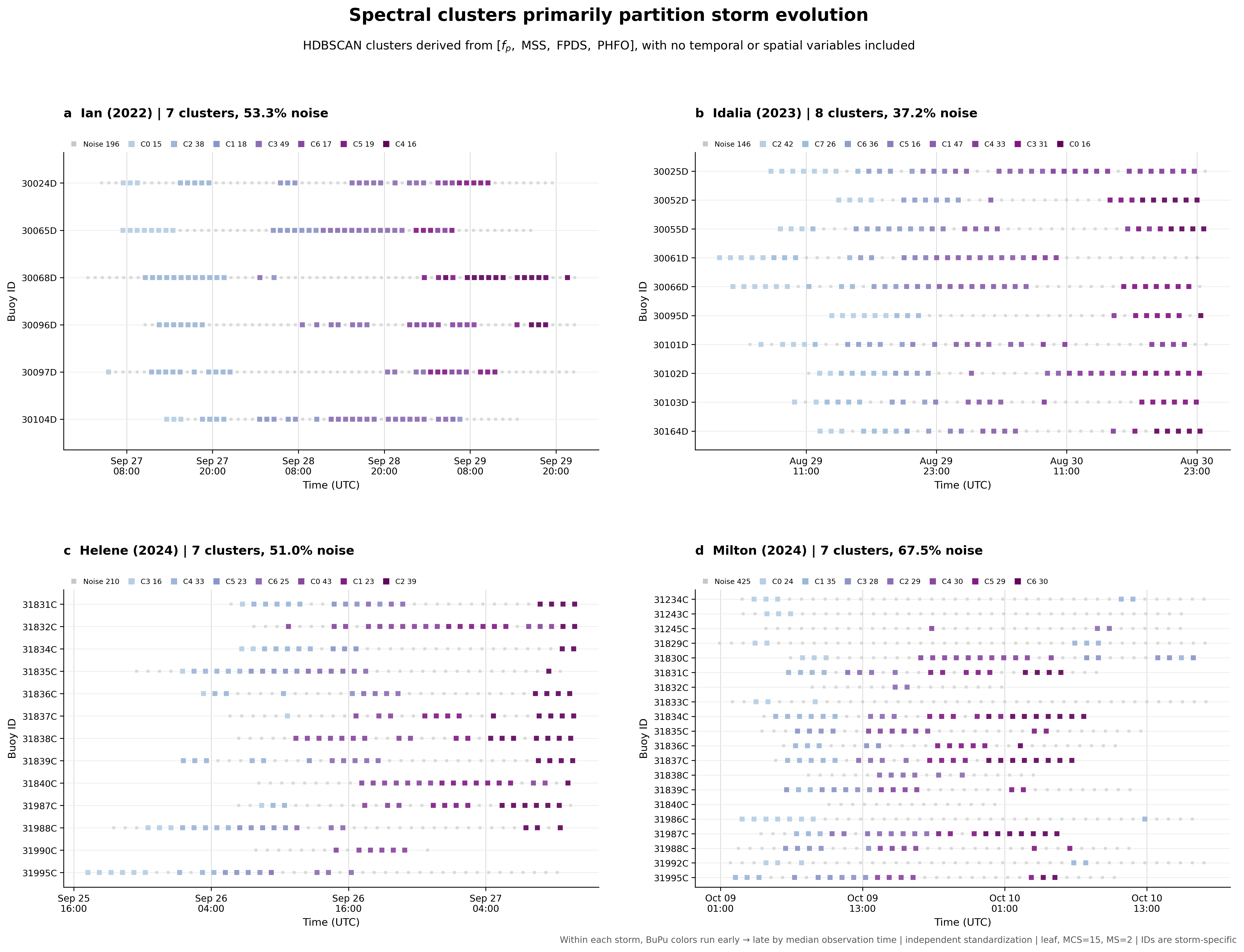Figure 2

12. Role in Chapter 1: this changes the conceptual model of the problem.
    • Reject the initial hypothesis that TC wave fields can be adequately described as a small number of discrete spectral regimes.
    • Replace it with a continuous-state / trajectory framework: observations occupy different positions along an evolving spectral manifold.
    • The temporal ordering provides the first evidence that wave history matters: spectra that appear similar are associated with where the wave field has come from and how it is evolving, not simply with a static instantaneous state.
    • This motivates the subsequent analyses of instantaneous forcing versus wind history, directional disequilibrium, and wave-memory metrics.
    • Chapter-level transition: If spectral variability is primarily continuous and evolutionary rather than categorical, the next question is what physical forcing and history determine position and motion along that continuum.

MAKE FIGURE 3: PCA structure of wave-state space Combine existing PCA loadings and PC1–PC2 physical-variable maps: A. PCA loadings B. fp C. MSS D. directional spread E. tail exponent (MOVE TO SUPPLEMENT: Existing marginal/PDF PCA figure.)

WRITE RESULT Report that PC1 is dominated by the inverse fp–MSS relationship, while PC2 primarily contrasts directional spreading with tail steepness. MSS and fp vary mainly along PC1, whereas directional spread and tail exponent retain substantial variability across both dimensions. Conclude that directional organization represents an additional degree of freedom in observed wave state. (ADD: Numerical loadings and explained variance.) (ADD ANALYSIS: Quantify the transverse variability rather than relying only on visual gradients.)

3.2 A common state space contains storm-specific trajectories

WRITE RESULT Show that storms occupy overlapping portions of the same low-dimensional manifold while tracing coherent, temporally evolving paths.

MAKE FIGURE 4: Shared Isomap manifold and storm trajectories A. Global Isomap colored by storm B. Colored by energetic/spectral-scale quantity C. Colored by directional spreading D–I. Individual storm trajectories colored by time (USE: PCA primarily for interpretable axes; Isomap primarily for nonlinear geometry/trajectories.) (MOVE TO SUPPLEMENT OR REPLACE: Existing PCA storm-trajectory figure.)

INSERT FOUR-PARAMETER TRAJECTORY RESULT

MAKE FIGURE 4: Four-parameter trajectory reconstruction. Show observed vs reconstructed trajectories for representative storms plus aggregate reconstruction performance across all storms.

(MOVE TO SUPPLEMENT OR REPLACE: Existing Idalia-only forcing/trajectory figure.) (ADD ANALYSIS: Make an all-storm version of the state-space dependence on wind speed, radius, and azimuth/quadrant.)

3.3 Instantaneous forcing explains energetic state better than directional state

WRITE RESULT Report instantaneous-only LOSO explained deviance: Hs 0.827 MSS 0.769 fp 0.662 Rhf 0.790 HFDS 0.180 FPDS 0.033 PHFO 0.069 State that instantaneous forcing provides substantial transferable skill for energetic/spectral-scale quantities but little skill for FPDS and PHFO.

MAKE FIGURE 5: Instantaneous-forcing predictive skill. Use a compact dot/bar plot across all seven responses, grouped into energetic/spectral-scale and directional quantities. (ADD: Selected GAM partial-dependence plots needed for physical interpretation.) (MAKE SUPPLEMENTARY FIGURE S4: Full instantaneous GAM diagnostics.) (ADD ANALYSIS: Evaluate whether differing measurement uncertainty/noise contributes to the skill contrast among response variables.)

3.4 Historical forcing preferentially explains directional wave-state properties

INSERT CURRENT SUMMARY RESULT Report: FPDS: 0.033 -> 0.181, DeltaD = +0.148 PHFO: 0.069 -> 0.165, DeltaD = +0.095 HFDS: 0.180 -> 0.230, DeltaD = +0.050 Contrast with smaller history increments for Hs, MSS, fp, and Rhf.

MAKE FIGURE 6: Instantaneous versus history-informed forcing skill.

Simplify the current summary figure: A. instantaneous vs combined LOSO skill B. DeltaD for all variables C. HFDS lag/timescale response D. FPDS lag/timescale response E. PHFO lag/timescale response

(MOVE TO SUPPLEMENT: Full seven-variable lag curves and complete best-model matrix if needed.) (KEEP: Held-out-storm uncertainty.) (CHECK ANALYSIS: Ensure history-model selection is nested appropriately inside LOSO validation; rerun within training folds if necessary.) (ADD ANALYSIS: Report storm-by-storm history skill changes for FPDS, PHFO, and HFDS.) (MAKE SUPPLEMENTARY FIGURE S5: Storm-specific history increments.)

4. DISCUSSION

4.1 Directional organization is an independent dimension of TC wave state

WRITE SYNTHESIS

Connect PCA/Isomap with instantaneous GAM results: energetic/spectral-scale variables organize the dominant axis, directional spreading contributes transverse variability, and instantaneous forcing predicts the former much better than the latter. (ADD: Relevant literature)

4.2 Directional state preferentially retains forcing-history information

WRITE SYNTHESIS

Explain that small history increments for Hs/MSS/fp/Rhf do not imply absence of memory. Instantaneous TC winds can proxy much of recent forcing because the wind field is autocorrelated. DeltaD measures additional historical information beyond that contemporaneous proxy.

State that this additional information is concentrated in directional quantities. (ADD ANALYSIS: Quantify wind autocorrelation over relevant history timescales.) (MAKE SUPPLEMENTARY FIGURE S6 OR MAIN-TEXT INSET: Wind autocorrelation vs lag.)

4.3 Dynamical interpretation of the state-space manifold

WRITE SYNTHESIS

Interpret the manifold as a state space through which the wave field evolves:

• contemporary forcing strongly constrains energetic/spectral-scale position;
• prior directional forcing contributes to evolution in the directional dimension;
• storms trace distinct trajectories through shared physically accessible states.

MAKE FIGURE 7: Conceptual synthesis

Create a schematic with an energetic/spectral-scale axis, a directional-organization axis, an evolving trajectory, instantaneous forcing associated mainly with energetic position, and directional history associated with directional evolution. Do not imply that the dynamical mechanism has been fully diagnosed.

4.4 Processes not resolved by the observational framework

WRITE

State that the historical predictors are simplified statistical representations and cannot isolate wind input Sin, nonlinear transfer Snl, dissipation Sds, propagation, or wave–current effects.

Use this limitation to motivate source-term-resolving spectral-wave modeling.

(OMIT FROM MAIN RESULTS: Local two-sheet/bimodality analysis unless it produces a clear result that materially changes the central argument.)

5. CONCLUSIONS

WRITE: ~4–6 concise findings in prose.

1. Multi-storm observations provide little evidence for stable discrete wave-state regimes and instead occupy a structured low-dimensional continuum.
2. Spectral scale/surface slope define the dominant axis while directional organization provides an additional degree of freedom.
3. Different TCs occupy a common state space but trace distinct trajectories through it.
4. Instantaneous forcing explains substantial held-out variance in Hs, MSS, fp, and Rhf but little in several directional quantities.
5. Historical forcing produces the largest independent skill gains for FPDS and PHFO, with a smaller but meaningful gain for HFDS.
6. Directional wave-state properties therefore retain information about prior directional forcing not contained in instantaneous forcing alone; dynamical modeling is needed to identify the responsible source-term processes.

PROPOSED MAIN FIGURES

Figure 1 — Dataset/storm observational coverage Figure 2 — HDBSCAN robustness summary Figure 3 — All storm cluster membership timeline Figure 4 — PCA state-space structure and physical-variable gradients Figure 5 — Shared Isomap manifold and individual storm trajectories Figure 6 — Four-parameter trajectory reconstruction Figure 7 — Instantaneous-only GAM skill Figure 8 — Historical-forcing skill increment and directional history dependence Figure 9 — Conceptual synthesis

PROPOSED SUPPLEMENT

Figure S1 — Extended HDBSCAN sensitivity Figure S2 — Isomap neighborhood-size sensitivity Table S1 — Complete forcing-history model grid Figure S3 — Full history lag/timescale curves Figure S4 — Full instantaneous GAM diagnostics Figure S5 — Storm-specific history skill Figure S6 — Wind autocorrelation versus lag Existing PCA marginal/PDF figure Existing PCA storm-trajectory figure, if replaced by Isomap Existing Idalia physical-forcing trajectory figure, if replaced by all-storm analysis

Notes:

\text{wave state}
\approx
\underbrace{\text{energy/scale}}_{f_p,MSS,R_{hf},H_s}
+
\underbrace{\text{directional breadth}}_{FPDS}
+
\underbrace{\text{inter-frequency directional disequilibrium}}_{PHFO}

Directional disequilibrium is multidimensional. Forcing history manifests both as changes in directional breadth within spectral bands and as directional separation between frequency bands.

spectral state constrains the possible directional state,
forcing history helps select the realized one

Road map:

1. TC wave fields are not a collection of equilibrium sea states. They continuously evolve through a structured state space, and HDBSCAN’s inability to recover robust categories is itself evidence against a discrete-regime description. The smooth gradients you see in the reduced state space support the same interpretation. 

2. The state space is organized by storm evolution. HDBSCAN knows nothing about time, yet the spectral clusters emerge in approximately chronological sequences across buoys. That means the spectral variables themselves contain information about the system’s evolution.

3. Therefore the wave field contains a record of previous forcing. This is where “wave memory” becomes more than a statistical predictor. The spectrum is effectively carrying information forward from earlier wind conditions.

4. That memory is not distributed equally across the spectrum. Bulk/energetic quantities appear closer to the instantaneous forcing, while directional and cross-frequency quantities retain substantially more information about prior forcing. That distinction is physically interesting: different portions or properties of the spectrum adjust on different timescales.

5. Therefore a single equilibrium descriptor such as $U_{10},H_s$, or wave age cannot uniquely specify the TC sea state. Even spectra occupying similar bulk sea-state space can retain systematically different high-frequency structure. (found explicitly in the spectral analysis)

6. The implication for air–sea interaction is potentially substantial. If MSS, directional spreading, alignment, and high-frequency structure depend on forcing history, then surface properties relevant to momentum exchange can also be path-dependent. You should phrase this as an implication rather than something this paper directly demonstrates unless you actually calculate stress/flux consequences.