Figures:
- Idalia quadrant composite spectra + alignment (wind-speed binned)
- High frequency energy fraction () vs MSS across Ian, Idalia and Milton
- Quadrant sensitivity analysis (stable vs boundary-sensitive samples)
Hypothesis before the figures
The earliest version of the hypothesis was built around a fairly simple picture of the wave field. We assumed that quantities like peak frequency, significant wave height, mean square slope and wind speed largely described the state of the sea surface. If two observations had similar values of these bulk parameters, then they should represent essential the same physical sea state.
As the work progressed, however, the HDBSCAN clustering, PCA and manifold learning analyses began to suggest something more interesting. Observations that appeared almost identical in terms of their bulk statistics sometimes occupied different locations within the reduced-dimensional state space. The most intriguing interpretation was that there might be two distinct families, or “sheets”, of sea states that could exist under nearly identical bulk forcing.
Initially, this idea looked surprisingly convincing. The lower sheet appeared to contain spectra with narrower directional spreading, relatively enhanced high frequency energy, and larger estimates of wave-supported stress, while the upper sheet exhibited broader spreading and comparatively weaker high frequency tails. It was an exciting possibility because it implied that the ocean might possess multiple dynamically stable spectral organizations even under nearly identical external forcing.
At that point, the project was moving toward a hypothesis that is summarized as:
Bulk sea-state parameters are insufficient because there are multiple discrete organizational states of the wave field
What the conference figures were testing
The objected had shifted by this time. I was no longer trying to demonstrate that storm-relative organization existed as that had already been shown repeatedly.
Instead, I was asking whether the two sheet interpretation remained physically meaningful one the analysis expanded beyond the original Idalia observations.
The conference figures acted as a stress test of the hypothesis.
- Could the apparent bifurcation survive when looking across multiple storms?
- Would the same separation appear when the spectra were composited differently?
- Would high frequency organization still separate into two populations once the sample size increased?
Figure 1: storm relative composite spectra
This first figure, showing the composite spectra and directional alignment organized by storm-relative quadrant and wind speed, ended up serving a different role that originally expected.
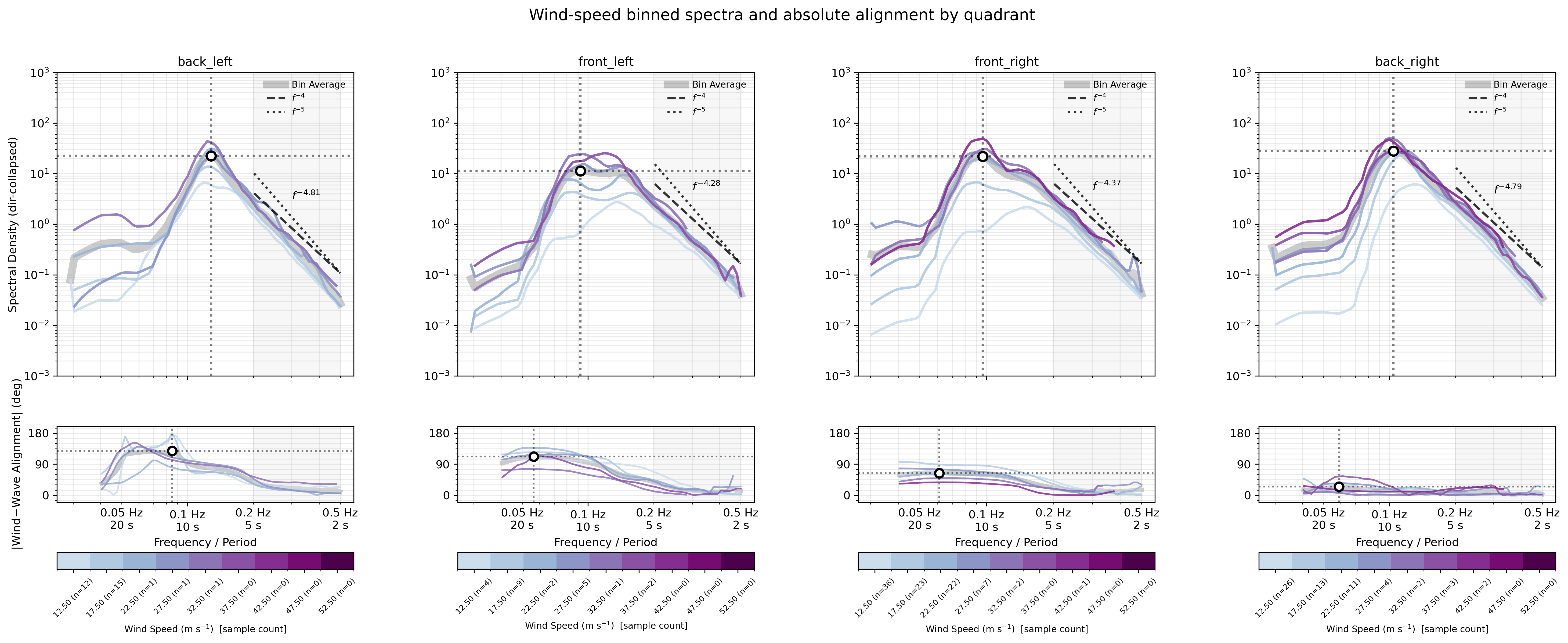
Originally, we viewed it primarily as another demonstration of storm relative differences. But after all of the previous work, that wasn’t really its contribution anymore.
Instead, it became something closer to a baseline description of the wave field.
It showed that once observations are grouped according to storm relative position, the spectra evolve in a remarkably coherent manner. As wind sped increases, the spectral energy shifts predictably, and the directional alignment curves evolve smoothly. There are no abrupt transitions between fundamentally different spectral states. Instead, the spectra appear to change continuously with both forcing and storm relative location.
This is actually an important observation because it establishes that much of the variability in the dataset can already be explained by known physical controls. The wave field is responding in a largely continuous way to changing wind forcing and storm relative geometry.
The figure itself therefore did not strengthen the two sheet hypothesis.
It established the background against which any additional organizational differences would have to be identified.
Figure 2: high frequency fraction vs MSS
This figure changed the interpretation.
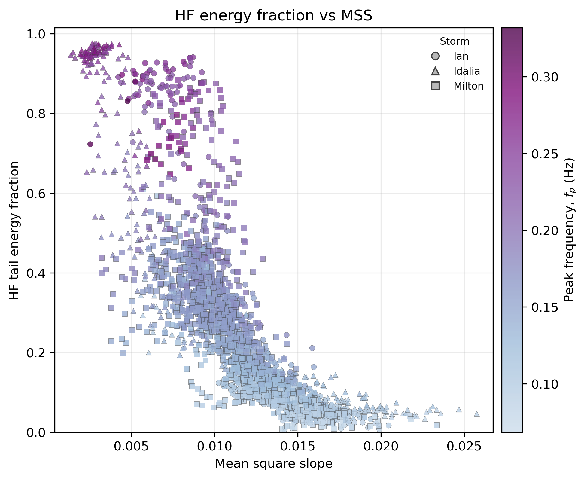
The expectation going into this analysis was that the two sheet hypothesis would manifest as two distinct populations occupying similar regions of bulk parameter space. In particular, we expected that observations with similar MSS would separate into two branches with systematically different high frequency energy fractions.
Instead, the relationship was surprisingly continuous.
As MSS increased, the relative contribution of high frequency energy decreased in a smooth and physically intuitive manner. Rather than separating into two clouds, the observations formed what looked much more like a continuum associated with wave development and spectral maturity.
At first this was disappointing because it weakened one of the strongest arguments for discrete spectral states. But after sitting with the results for a while, it actually revealed something more interesting.
It suggested that energy content itself is largely governed by the same continuous physical processes we already understand.
- Wave growth redistributes energy gradually.
- Spectral maturity evolves gradually.
- Mean square slope evolves gradually.
Nothing in the figure indicated multiple discrete solutions.
This was an important conceptual shift because it suggested that if multiple organizational states exist, they are probably not distinguished primarily by how much high frequency energy is present.
Instead, they are more likely distinguished by how that energy is organized. This is a fundamentally different hypothesis.
Figure 3: quadrant sensitivity
The quadrant analysis depends on assigning each observation to a storm relative region. Any reviewer could reasonably ask whether the observed differences were artifacts of uncertain quadrant assignments, particularly near the storm center or during periods of rapid track curvature.
Rather than ignoring this uncertainty, it was quantified directly.
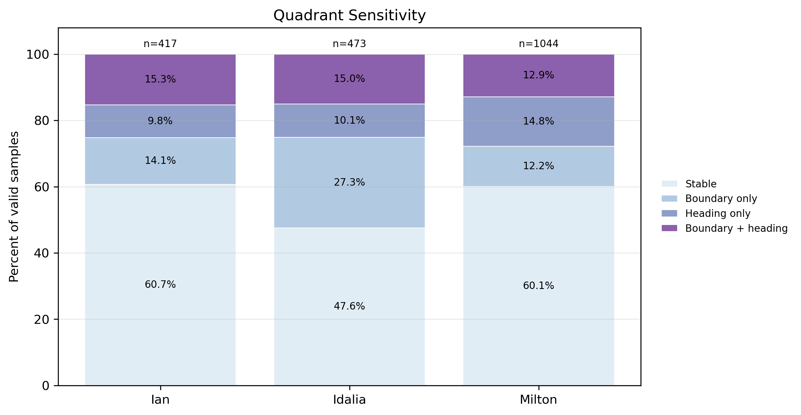
The sensitivity analysis demonstrated that the ambiguity was localized and understandable. Most uncertainty occurred precisely where we would expect it physically: near quadrant boundaries or during periods when the storm heading changes rapidly.
The stable observations continued to show the same qualitative behavior as the full dataset.
This strengthened the credibility of the earlier composite analysis. The patterns were not simply emerging because observations had been arbitrarily assigned to quadrants. They persisted even after accounting for classification uncertainty.
While this figure did not directly influence the physical hypothesis, it substantially strengthed the methodological foundation of the work.
Emergent hypothesis
The evolution was from discrete spectral states toward additional degrees of freedom in spectral organization
The evidence increasingly suggested that bulk sea quantities evolve as continuous variables although not as tightly constrained as we once thought. It also indicates that two spectra with nearly identical MSS may differ in how tightly that energy is aligned with the local wind.
The peak region and the high frequency tail can become partially decoiupled, with the tail responding more directly to the instantaneous forcing while the peak retains memory of the integrated wave history.
Those differences are subtle, yet they are precisely the properties that should matter for air sea momentum transfer, since the shortest wind waves dominate the form stress acting on the atmosphere.
Storm-relative forcing explains the dominant evolution of the wave field. Bulk metrics describe much of that evolution and behave largely continuously. However, those bulk quantities do not uniquely specify the detailed structure of the spectrum. There remains an additional layer of variability associated with the directional organization of the high-frequency tail, its alignment with the wind, and the partitioning of energy across scales. These organizational differences are subtle enough that they are easily hidden by integrated metrics like MSS, yet they may be precisely the part of the spectrum that controls wave-supported stress, drag, and ultimately air–sea coupling.
Future hypothesis
Our previous analyses demonstrated that storm relative forcing organizes the evolution of the wave spectrum and that bulk sea state properties such as mean square slope (MSS), peak frequency, and high-frequency energy evolve largely continuously with increasing wind forcing. These results suggest that much of the observed spectral variability can be explained by the magnitude and history of the forcing alone. However, they also indicate that bulk quantities do not uniquely describe the directional organization of the high-frequency tail.
Based on this, I hypothesize that high frequency directional organization represents an additional degree of freedom that modulates the efficiency of air-sea momentum transfer beyond what is captured by bulk sea state metrics alone. Specifically, for a given forcing magnitude (e.g., wind speed), variability in MSS, inferred friction velocity (), or other stress related quantities should be partially explained by the alignment of the high frequency tail with the local wind.
In other words, two sea states experiencing similar wind forcing may develop different levels of wave supported stress because the short wave energy is organized differently in directional space.
Furthermore, I hypothesize that the influence of high frequency directional organization is itself a function of forcing magnitude. At low wind speeds, the high frequency tail is relatively weak and contributes little to variability in stress related quantities. As forcing increases and the high frequency tail becomes increasingly important to air-sea momentum exchange, directional organization should explain a progressively larger fraction of the remaining variability. At sufficiently high forcing, where MSS, drag or wave supported stress begin to saturate due to wave breaking and other nonlinear processes, the influence of directional organization may likewise diminish or plateau. Thus, the explanatory power of high frequency alignment is expected to vary systematically across the forcing regime rather than remain constant.
Next steps
The next stage of this work is to quantify the relationship between high frequency directional organization and stress-related quantities while explicitly controlling for forcing magnitude.
The first step is to define a robust metric describing the alignment of the high frequency tail relative to the local wind direction. This metric should represent the directional organization of the short-wave field independently of its total energy content and should be calculated consistently across all observations.
Using this metric, the analysis will then investigate whether high-frequency alignment explains residual variability in quantities such as MSS, inferred friction velocity (), or wave-supported stress after accounting for wind speed and other bulk descriptors. Rather than examining simple correlations across the entire dataset, the analysis will condition on forcing magnitude by either binning observations by wind speed or by fitting statistical models that include an interaction between wind speed and the alignment metric.
Within each forcing regime, the amount of variance explained by high-frequency alignment will be quantified using measures such as regression slope, partial , or reductions in prediction error. The resulting relationship between forcing magnitude and explanatory power will reveal whether directional organization becomes increasingly important as winds strengthen and whether its influence eventually saturates at the highest wind speeds.
If successful, this analysis would demonstrate that high-frequency directional organization provides predictive information beyond traditional bulk sea-state metrics. Rather than replacing variables such as MSS or peak frequency, the alignment metric would serve as an additional descriptor of the wave field that helps explain differences in wave-supported stress and air-sea momentum exchange among sea states that are otherwise similar according to conventional bulk measures.
Forcing magnitude → HF-tail organization → stress → observed MSS / wave growth.
In this framework, MSS and are not the primary targets but rather observable consequences of how efficiently the high frequency tail couples the atmosphere to the ocean. If the analysis supports that chain, it becomes a much more mechanistic story than simply finding another empirical predictor.