Overall figure description
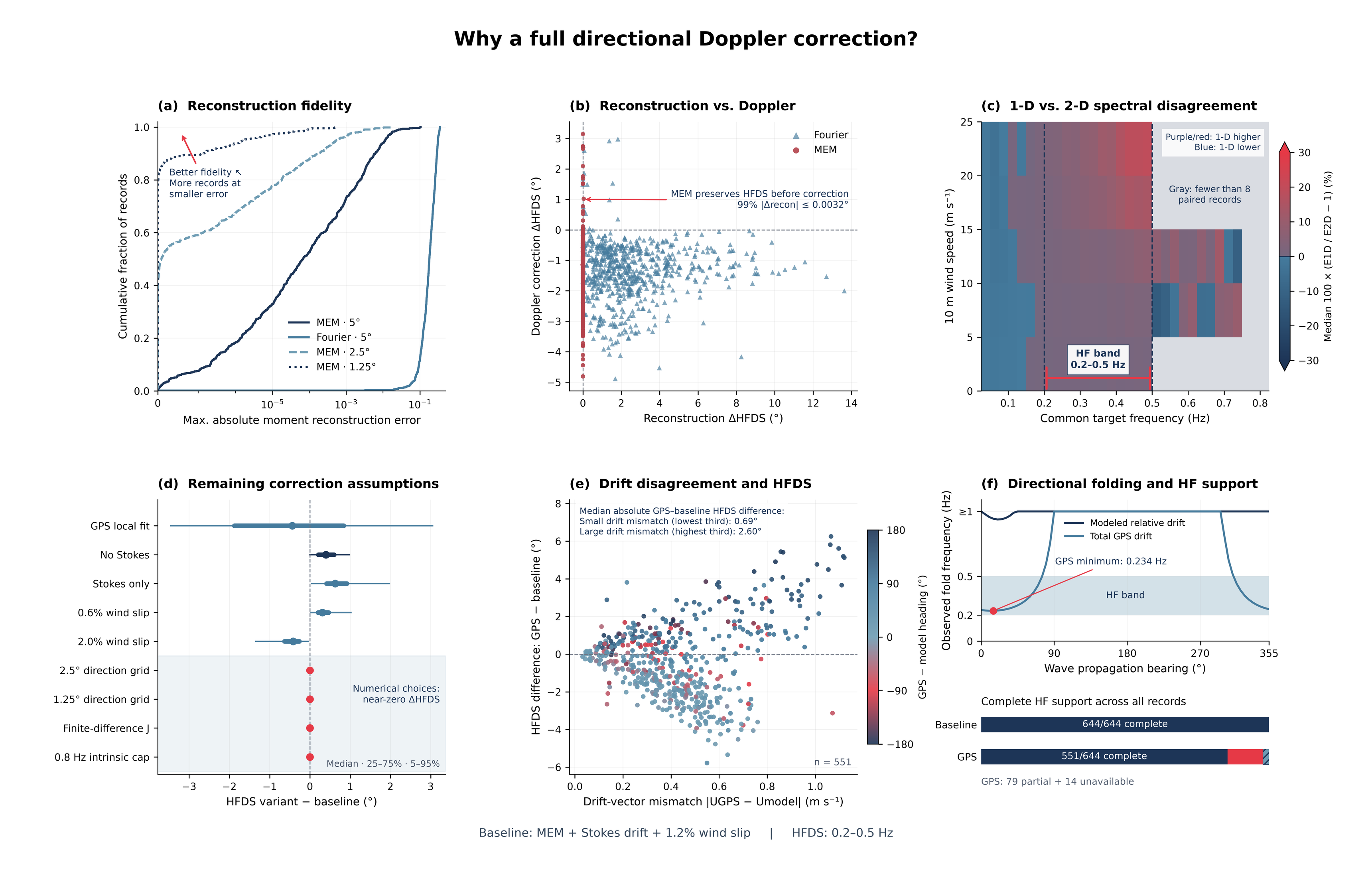
This figure evaluates the methodological choices used for the full directional Doppler correction of the Spotter spectra. The baseline method uses a maximum entropy (MEM) reconstruction of , a 2.5° directional grid, a full two-dimensional Doppler transformation, and a modeled drift vector consisting of Stokes drift plus 1.2% wind slip. HF directional spread (HFDS) is evaluated over 0.2–0.5 Hz. A finer 1.25° MEM grid is included as a numerical convergence test, rather than as a separate physical model, because grid refinement changes only how finely the MEM solution is sampled and does not add new directional information beyond the measured moments.
The panels distinguish several different sources of disagreement. Reconstruction error is defined relative to the original Spotter-supplied directional moments, while HFDS sensitivities are defined relative to the MEM + Stokes + 1.2% wind baseline. The figure therefore separates changes introduced by reconstruction of , by using a 1-D rather than 2-D Doppler treatment, by numerical implementation choices, and by changing the assumed drift vector.
A) Reconstruction fidelity
This panel shows the cumulative distribution of the maximum absolute discrepancy between the directional moments implied by the reconstructed and the original moments supplied by the buoy. Curves farther toward the upper-left indicate that a larger fraction of records reproduce the measured moments with small error.
MEM reproduces the supplied directional information substantially more faithfully than the Fourier reconstruction. Refining the MEM grid from 5° to 2.5°, and then to 1.25°, progressively reduces the already small numerical reconstruction residual. However, this refinement represents improve quadrature/sampling of the same MEM solution, not additional observational directional resolution. Together with panel (d), the convergence of HFDS between 2.5° and 1.25° supports 2.5° as the production grid, with 1.25° retained as a convergence test.
B) Reconstruction vs Doppler correction
The x-axis shows the change in HFDS introduced only by reconstructing the directional distribution, relative to HFDS calculated directly from the original directional moments. The y-axis shows the additional HFDS change produced when the Doppler transformation is subsequently applied.
MEM introduces essentially no HFDS change before correction, so changes after reconstruction can be attributed to the moving-frame transformation itself. Fourier reconstruction can alter HFDS by several degrees before Doppler correction is applied, mixing estimator effects with the physical reference-frame correction. This supports MEM as the preferred reconstruction method because it preserves the directional statistic being corrected.
C) 1-D vs 2-D spectral disagreement
This panel compares the archived 1-D mean-direction correction with the full 2-D directional treatment while holding the other correction choices fixed. Each wind–frequency bin shows so positive values indicate greater energy in the 1-D result, negative values indicate less, and gray bins contain too few paired observations for a stable comparison.
The disagreement is structured rather than random and is particularly evident within the 0.2–0.5 Hz HF band and at stronger winds. Because Doppler shift depends on the directional projection , assigning all energy at a given frequency a single mean propagation direction produces systematic differences when the actual directional distribution is broad. This supports the full 2-D correction as the physically appropriate treatment for directional and high-frequency quantities.
The 1-D method assumes that all energy at a given frequency propagates in the single mean wave direction. When that mean direction is reasonably aligned with the buoy drift, this assigns nearly the same large projected drift speed to the entire frequency bin. In reality, the energy is spread over a range of directions, many of which have smaller along-wave projections and therefore experience weaker Doppler shifts.
D) Remaining correction assumptions
Each row shows the distribution of where the baseline is MEM + Stokes drift + 1.2% wind slip on the 2.5° directional grid. Points show medians, with the wider intervals representing the central and outer portions of the paired-record distribution.
The purely numerical choices produce essentially zero change in HFDS. In particular, refining the directional grid from 2.5° to 1.25° has negligible effect on the final HFDS, even though panel (a) shows a further reduction in the already small moment-reconstruction residual. This demonstrates that HFDS has converged by 2.5°, supporting its use as the production resolution rather than paying the additional computational cost of a 1.25° grid that adds numerical precision but no meaningful change to the science result.
Changes to the physical drift assumptions produce larger but still generally modest shifts, while replacing the modeled drift with GPS generates a much broader response. The panel therefore shows that the result is insensitive to numerical tuning but meaningfully sensitive to the physical drift-vector assumption.
E) Drift disagreement and HFDS
The x-axis is the magnitude of the vector difference between total GPS velocity and the modeled drift, and the y-axis is the resulting HFDS difference, Point color indicates the difference between the GPS and modeled drift headings.
As the two drift vectors become more different, the corrected HFDS solutions increasingly diverge. The median absolute GPS–baseline HFDS difference grows from about for the lowest third of drift mismatch to for the highest third. This demonstrates that GPS is not simply a more precise estimate of the same correction velocity, it represents materially different motion and should therefore be treated as an alternative frame/drift sensitivity rather than automatically replacing the modeled relative-drift estimate.
F) Directional folding and HF support
The upper panel shows the observed frequency at which the Doppler mapping becomes non-invertible as a function of wave propagation direction. The modeled relative drift keeps this fold above the 0.2–0.5 Hz analysis band for essentially all directions, whereas the larger total GPS velocity can push the fold into the HF band, reaching a minimum of about 0.234 Hz.
Beyond the fold, one observed encounter frequency can correspond to more than one intrinsic frequency, so that portion of the directional spectrum cannot be uniquely recovered. The lower panel shows the practical consequence: the baseline retains complete HF support for all 644 records, whereas the GPS treatment retains complete support for 551 records, with additional records only partially supported or unavailable. This supports using the modeled Stokes + 1.2% wind drift as the operational baseline and retaining GPS as a sensitivity test rather than the default intrinsic correction.
Overall conclusions
Taken together, the diagnostics support MEM + full 2-D Doppler correction + a 2.5° directional grid + modeled Stokes drift and 1.2% wind slip as the operational baseline. MEM preserves the measured directional moments, the 2-D treatment avoids the systematic approximation introduced by collapsing the directional spectrum to a mean direction, and refinement from 2.5° to 1.25° confirms numerical convergence without materially changing HFDS. The remaining numerical implementation choices have negligible influence, whereas the dominant uncertainty lies in the physical drift-vector definition. Total GPS drift produces substantially different directional corrections and, in some cases, makes the HF inverse mapping non-unique.