Lead-Time Sensitivity of Buoy-Constrained TC Track Correction

Sensitivity-analysis objective

This sensitivity analysis evaluates whether the HF-tail track correction depends strongly on the temporal window used to represent the wind forcing. The goal is to identify a correction window that improves storm-relative spectral organization across storms, remains stable in independent holdout testing, and avoids introducing large or physically implausible changes to the underlying best-track trajectory. The analysis also tests whether the selected correction produces robust quadrant assignments and interpretable wind–wave alignment patterns for the subsequent storm-relative analysis.

Lead-Time Sensitivity of Directional Agreement and Track Geometry

Among the individual objective components, the directional matching term shows the clearest response when the wind forcing is shifted from concurrent conditions to a 60-minute lead. The rotation, ranking, and other geometric contributions remain broadly consistent between the two experiments, indicating that the optimizer recovers nearly the same storm-center evolution in both cases. The improvement in the total objective therefore arises primarily from better agreement between the modeled storm-relative wind direction and the observed high-frequency wave orientation, rather than from a substantially different corrected track.

The displacement diagnostics support the same interpretation. The 60-minute lead changes the temporal phasing of the center correction but produces only modest changes in its overall magnitude and geometry. The corrected track remains close to the no-lead solution and primarily introduces small along-track adjustments, with resulting quadrant changes concentrated near existing boundaries. Thus, the lead-time experiment is not exploiting additional geometric freedom; it is refining the timing relationship between the evolving wind field, storm position, and high-frequency wave response.

Relative to the no-lead experiment, the 60-minute lead produces the largest observed reduction in directional error while preserving the broader track structure. This is consistent with a finite adjustment time of the high-frequency wave field rather than an instantaneous response to the local wind. The result should not be interpreted as identifying an exact 60-minute physical response timescale, but it supports the use of a temporally offset forcing field and motivates the selected lead for the corrected storm-relative analysis.

The subsequent holdout experiment provides an independent validation of this choice: the improvement associated with the 60-minute lead persists when evaluated using observations excluded from the fitting procedure. Together with the stable track geometry and improved quadrant composites, this indicates that the selected lead captures a reproducible timing relationship rather than an in-sample optimization artifact.

60 min lead quadrant analysis

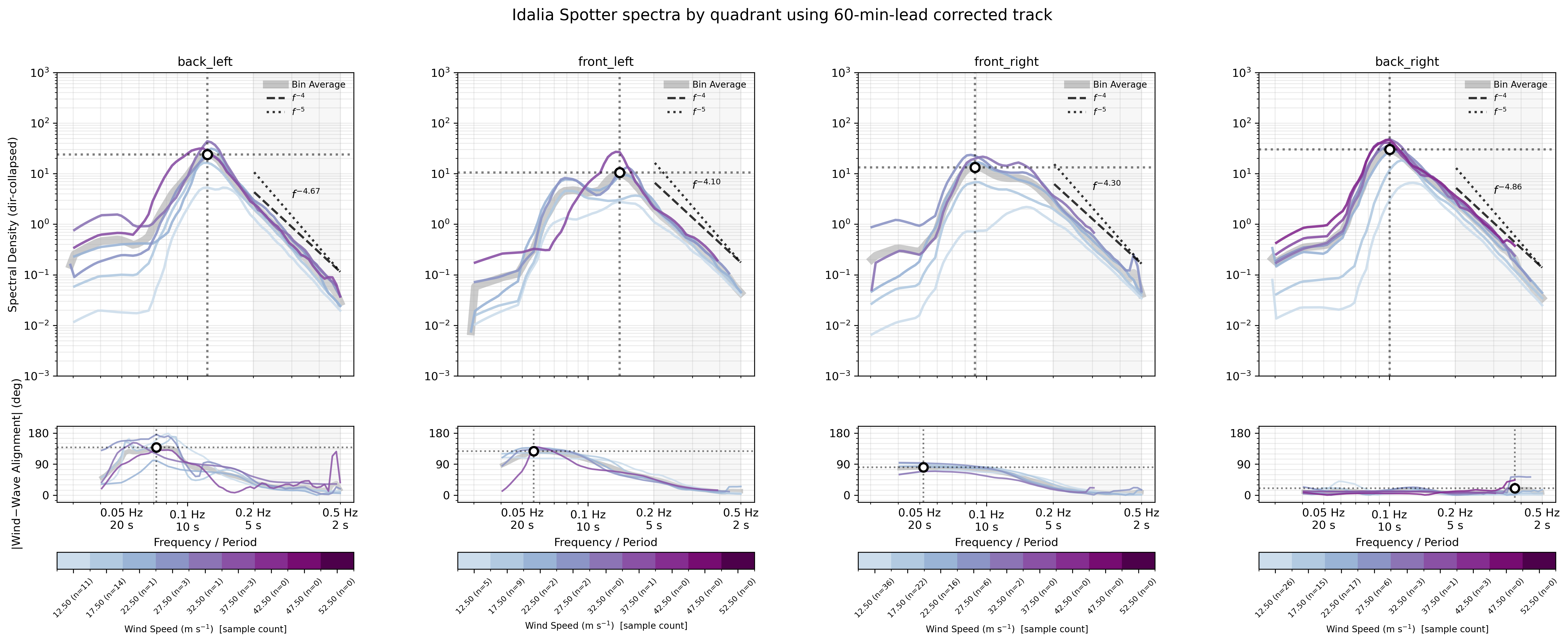
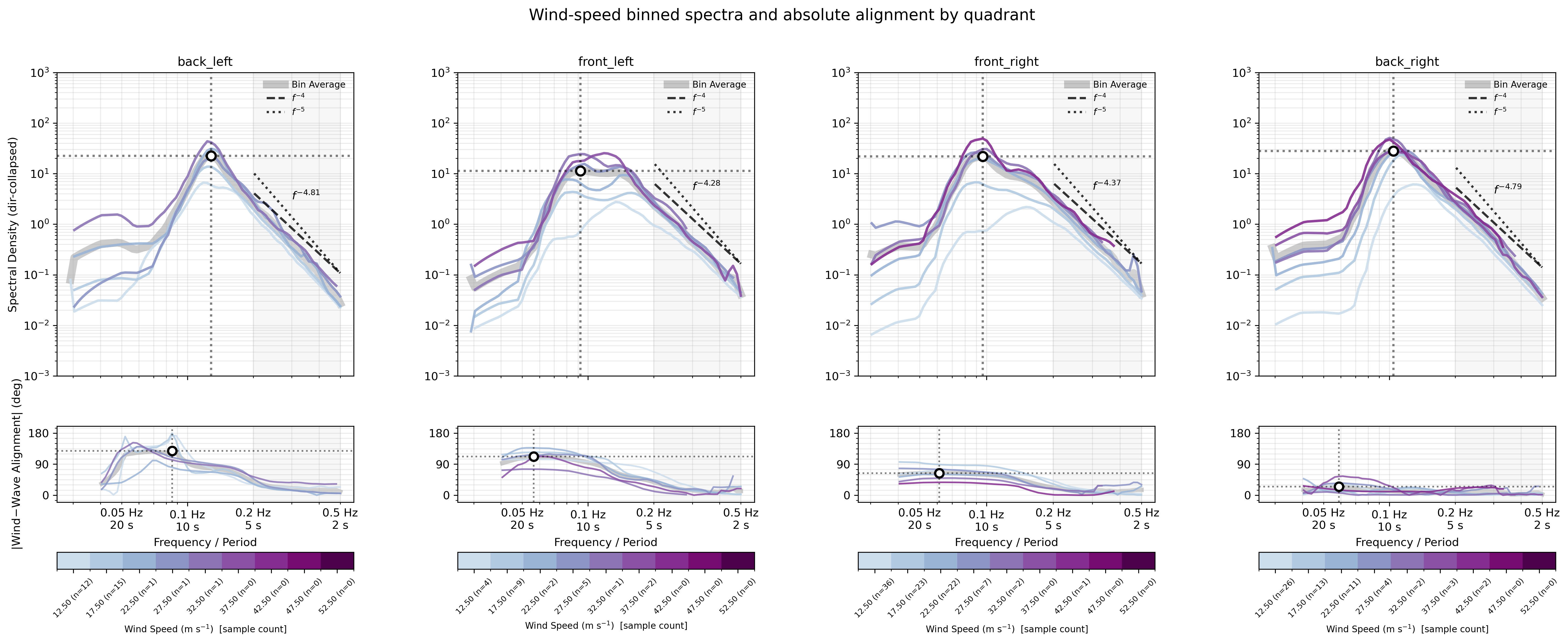
Using the 60-minute-lead corrected track improves the coherence of the quadrant-composited wind–wave alignment while largely preserving the spectral evolution. The clearest improvements occur in the front-left, front-right, and back-right quadrants, where the alignment curves form smoother and more consistent frequency dependent trends. The back-left quadrant remains more variable, particularly in the high-frequency tail. Some differences in the high-wind composites also reflect the reassignment of observations between quadrants under the corrected track.

The near-invariance of the spectral shapes indicates that the correction primarily improves the storm-relative reference frame rather than altering the observed wave evolution. Alternative energy-weighted and frequency-weighted alignment objectives produced nearly identical corrected tracks and did not further improve quadrant coherence. The 60-minute-lead correction was therefore retained, while the remaining back-left variability motivates further investigation of quadrant-dependent forcing histories rather than being interpreted as evidence of track-correction failure.

60 min lead

No lead

HF-tail track-correction timing experiment

To determine the wind interval most appropriate for estimating the high-frequency (HF) tail track correction, a buoy-level holdout experiment was performed across Hurricanes Ian (2022), Idalia (2023), Helene (2024), and Milton (2024). The experiment was designed to evaluate the timing of the track correction independently of the wind interval used for the final spectral comparison. For every candidate configuration, the corrected spectra were evaluated against the concurrent Spotter averaging interval, $[t-30,t]$. Thus, the experiment tested whether using earlier winds to estimate the track correction improved prediction of the HF-tail direction observed during the concurrent 30-minute measurement period.

Seven candidate track-correction intervals were considered. Each interval was a 30-minute wind average displaced progressively backward in time relative to the end timestamp t:

$[t-30,t],[t-45,t-15],[t-60,t-30],[t-75,t-45],[t-90,t-60],[t-105,t-75],[t-120,t-90]$.

These intervals correspond to nominal track-correction leads of 0, 15, 30, 45, 60, 75, and 90 minutes, respectively. Because Spotter timestamps represent the end of the preceding 30-minute spectral averaging interval, the 30-minute-lead configuration, $[t-60,t-30]$, uses the wind interval immediately preceding the observation interval rather than winds concurrent with it.

For each storm and candidate lead, the track-correction model was fitted using a withheld-buoy split and evaluated only on observations from buoys excluded from model fitting. This prevented observations from the same buoy from contributing to both model estimation and validation and therefore tested whether the timing choice generalized spatially across independent buoy trajectories. All candidate corrections were scored using the same concurrent $[t-30,t]$ wind reference, so differences among configurations were attributable to the wind timing used to calculate the track correction rather than to differences in the evaluation target.

Performance was quantified using three complementary held-out metrics: circular directional root-mean-square error,

${\mathrm{RMSE}}_{\theta }=\sqrt{\frac{1}{N}{\sum }_{i=1}^N\Delta {\theta }_i^2}$,

the improvement in directional RMSE relative to the uncorrected spectra,

$\Delta \mathrm{RMSE}={\mathrm{RMSE}}_{\mathrm{raw}}-{\mathrm{RMSE}}_{\mathrm{corrected}}$,

and the fraction of held-out observations whose absolute circular directional error was less than $30^{\circ }$. Aggregate held-out RMSE, mean absolute error, and median absolute error were also calculated across all storms. In addition, the distribution of per-observation RMSE improvement was examined to ensure that aggregate performance was not produced by a small number of unusually large improvements. A metric-winner count summarized how often each timing configuration produced the best result across the four storms and five evaluated performance criteria.

Timing-selection results

The 30-minute-lead configuration, $[t-60,t-30]$, produced the strongest and most consistent held-out performance. It yielded the lowest aggregate directional RMSE, approximately $19.8^{\circ }$, together with the lowest aggregate mean absolute error, $15.2^{\circ }$, and median absolute error, $12.3^{\circ }$. Its per-observation improvement distribution was also shifted toward positive values, indicating that the aggregate gain was broadly distributed rather than being controlled by a small subset of cases.

The 30-minute lead produced the minimum storm-specific held-out RMSE for Ian, Idalia, and Helene:

$14.6^{\circ },23.9^{\circ },\text{and}21.1^{\circ }$,

respectively. For Milton, the minimum RMSE of $19.2^{\circ }$ occurred at both the 15- and 30-minute leads to the displayed precision. The 30-minute lead also generated the largest RMSE improvement relative to the raw spectra for Ian, $4.2^{\circ }$, and Helene, $2.2^{\circ }$, and was effectively tied for the best result in Idalia. Milton showed its largest improvement at the 15-minute lead, $3.6^{\circ }$, with the 30-minute lead close behind at $3.5^{\circ }$.

The fraction of observations within $30^{\circ }$ was similarly favorable for the 30-minute configuration. It reached 0.98 for Ian, 0.78 for Idalia, 0.88 for Helene, and 0.90 for Milton. Although several leads produced numerically similar fractions for individual storms, the 30-minute lead was the most consistently competitive across all storms and metrics.

This consistency was reflected in the metric-winner count: the $[t-60,t-30]$ configuration accumulated 15 wins, whereas every other candidate interval produced at most one win. The 75-minute lead produced no metric wins. The relatively flat performance surrounding the optimum indicates that the correction is not extremely sensitive to small timing perturbations; nevertheless, the repeated held-out advantage of the 30-minute lead provides a clear empirical basis for selecting it.

Accordingly, the final processing workflow estimated the HF-tail track correction from winds averaged over

$[t-60,t-30]$,

while retaining the concurrent $[t-30,t]$ winds for spectral evaluation, Doppler correction, and subsequent physical analysis. This choice is also temporally consistent with the Spotter sampling convention: the correction is based on the 30-minute forcing interval immediately preceding the 30-minute wave-spectrum observation interval.

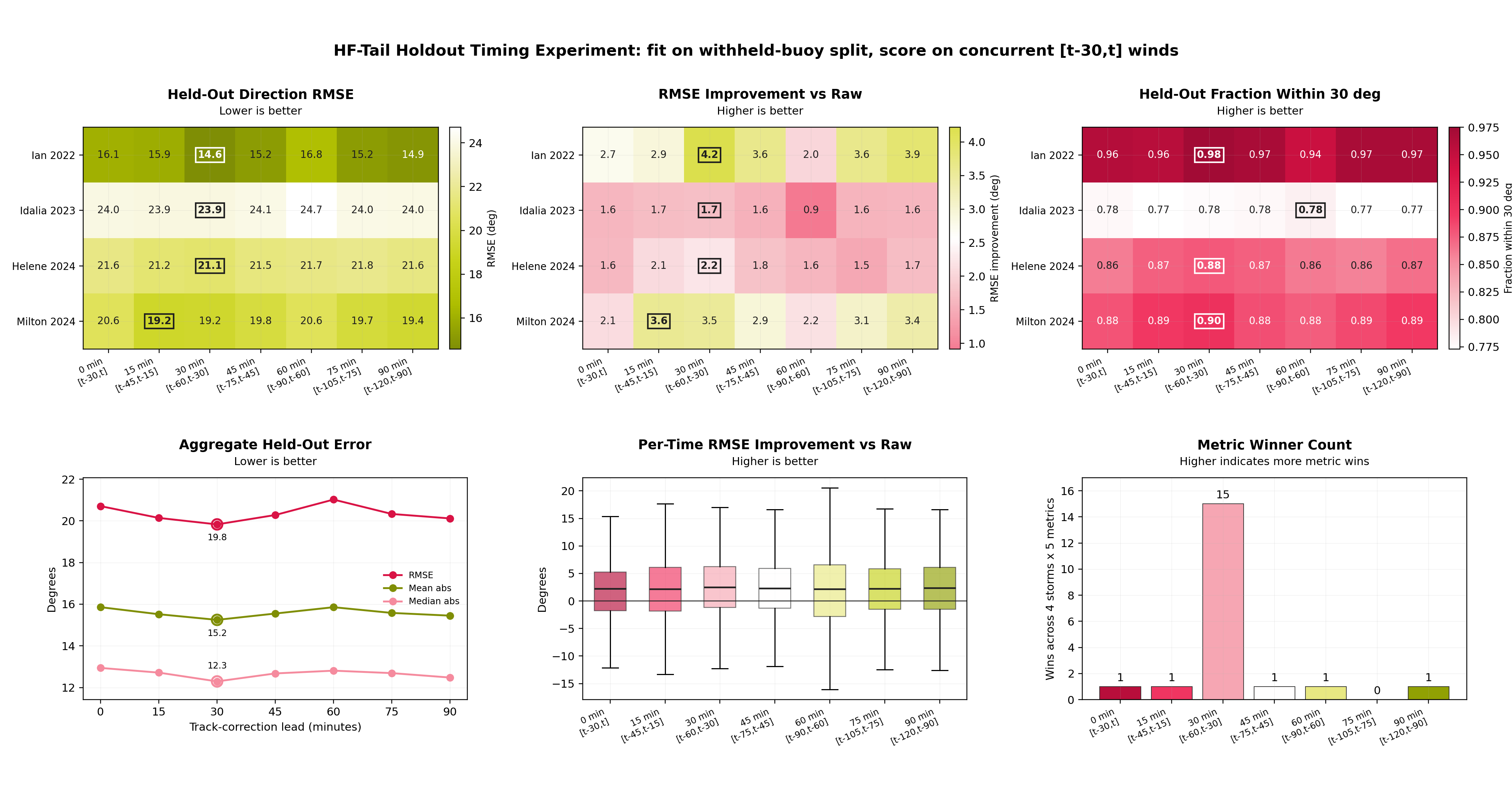
Held-out buoy timing experiment used to select the wind interval for the HF-tail track correction. Corrections derived from seven progressively lagged 30-minute wind windows were fitted using a withheld-buoy split and evaluated against concurrent $[t-30,t]$ winds for four tropical cyclones. The $[t-60,t-30]$ interval (30-minute lead) produced the lowest aggregate directional RMSE, mean absolute error, and median absolute error and won 15 of the 20 storm–metric comparisons, supporting its use in the final processing workflow.

HF-tail corrected storm tracks

The HF-tail correction introduces relatively small, along-track adjustments to the best-track position rather than large cross-track displacements. The resulting quadrant transitions are therefore concentrated near quadrant boundaries, which is consistent with correcting the storm center timing and along-track phase while preserving the broader storm trajectory. This provides a useful bridge between the lead-time diagnostics and the corrected quadrant composites: the selected t-60 to t-30 min correction changes classifications primarily where they are most sensitive, without reorganizing the storm-relative geometry wholesale.

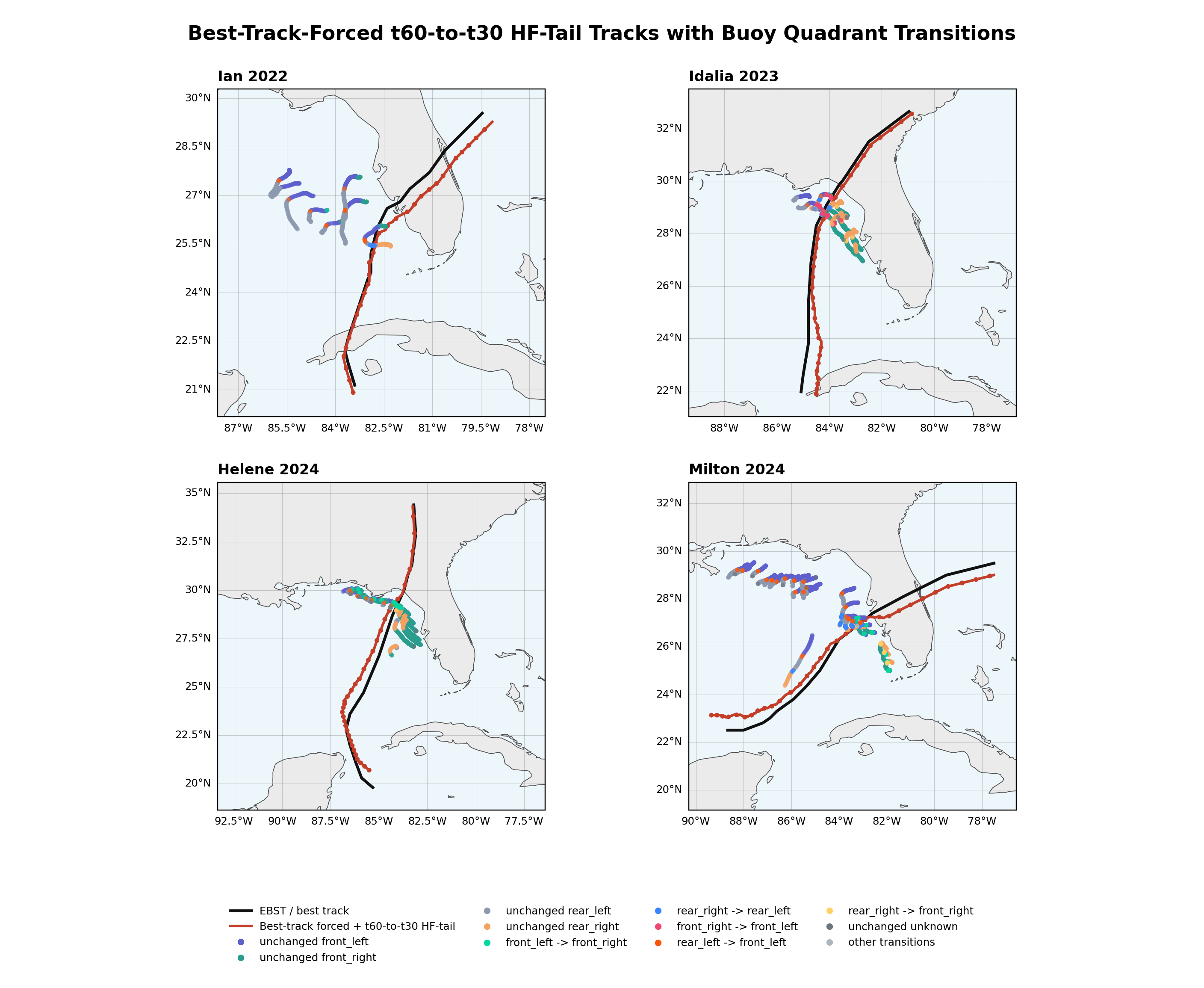
Comparison of the EBST best track (black) and the best-track-forced HF-tail-corrected track using the t-60 to t-30 min forcing window (red) for Ian, Idalia, Helene, and Milton. Colored buoy trajectories indicate whether storm-relative quadrant assignments remain unchanged or transition under the corrected track. Most changes occur near quadrant boundaries, consistent with modest predominantly along-track adjustments rather than large changes to the storm trajectory.

Validation of the storm-relative track correction

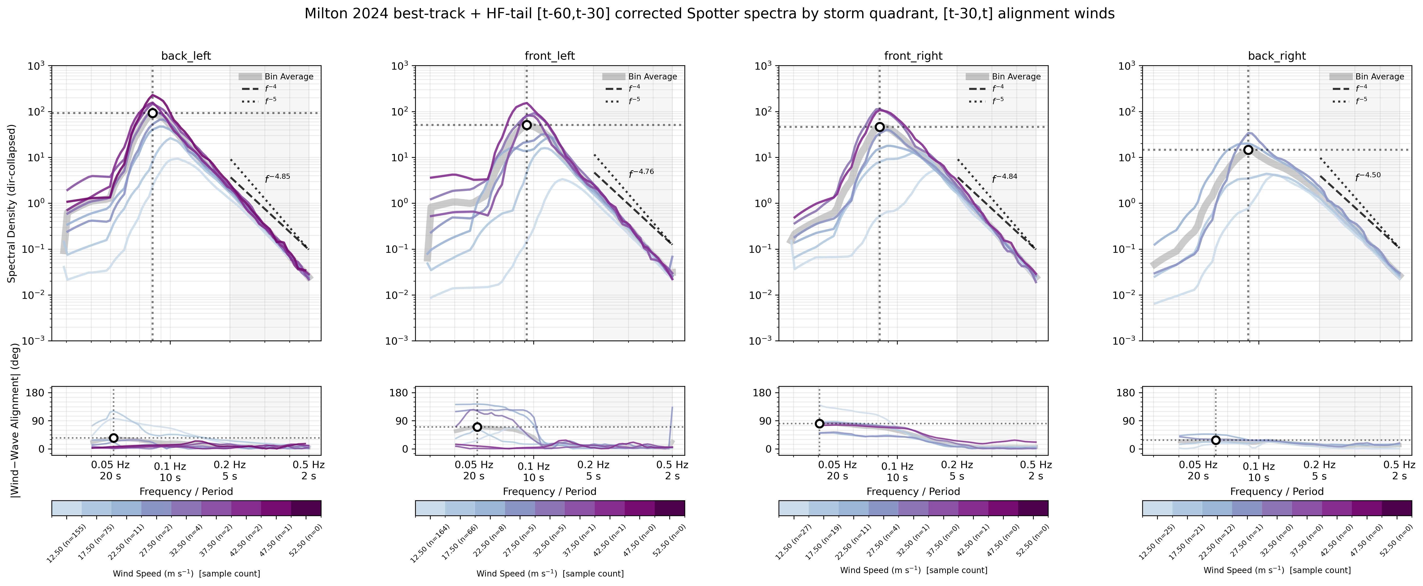
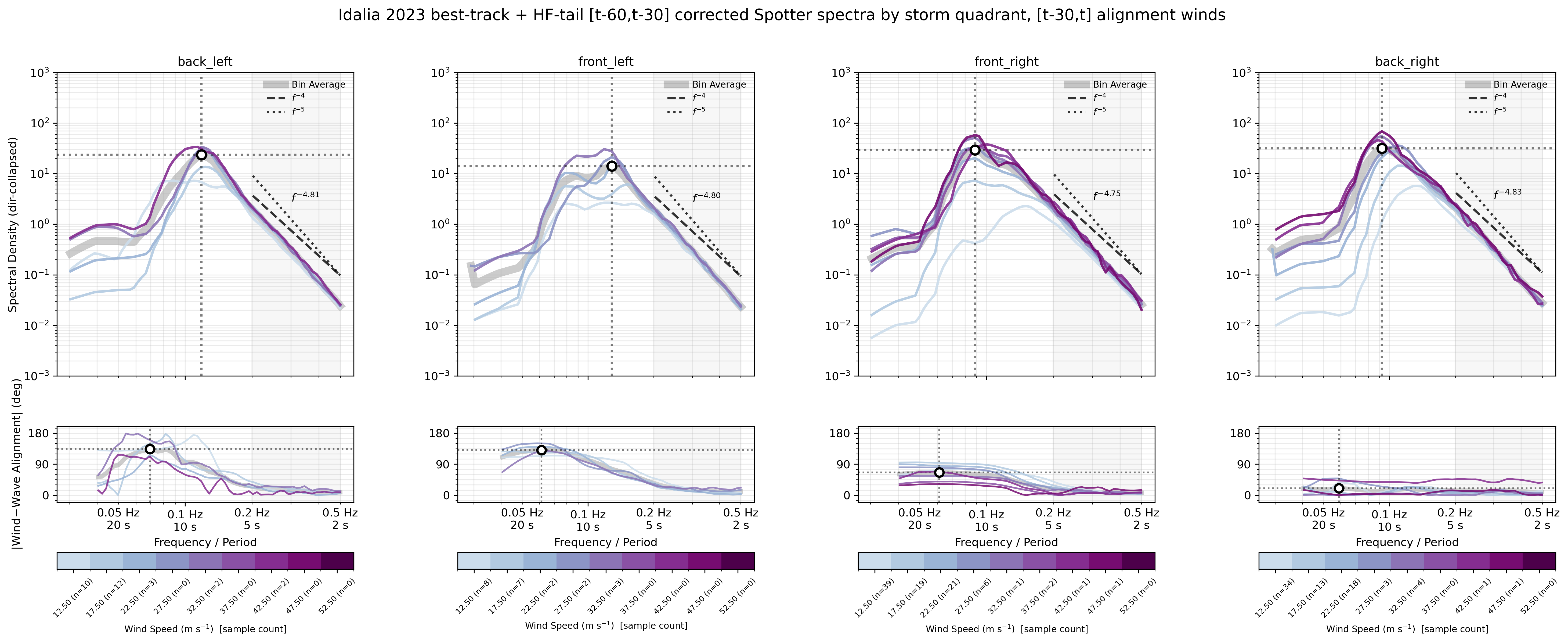
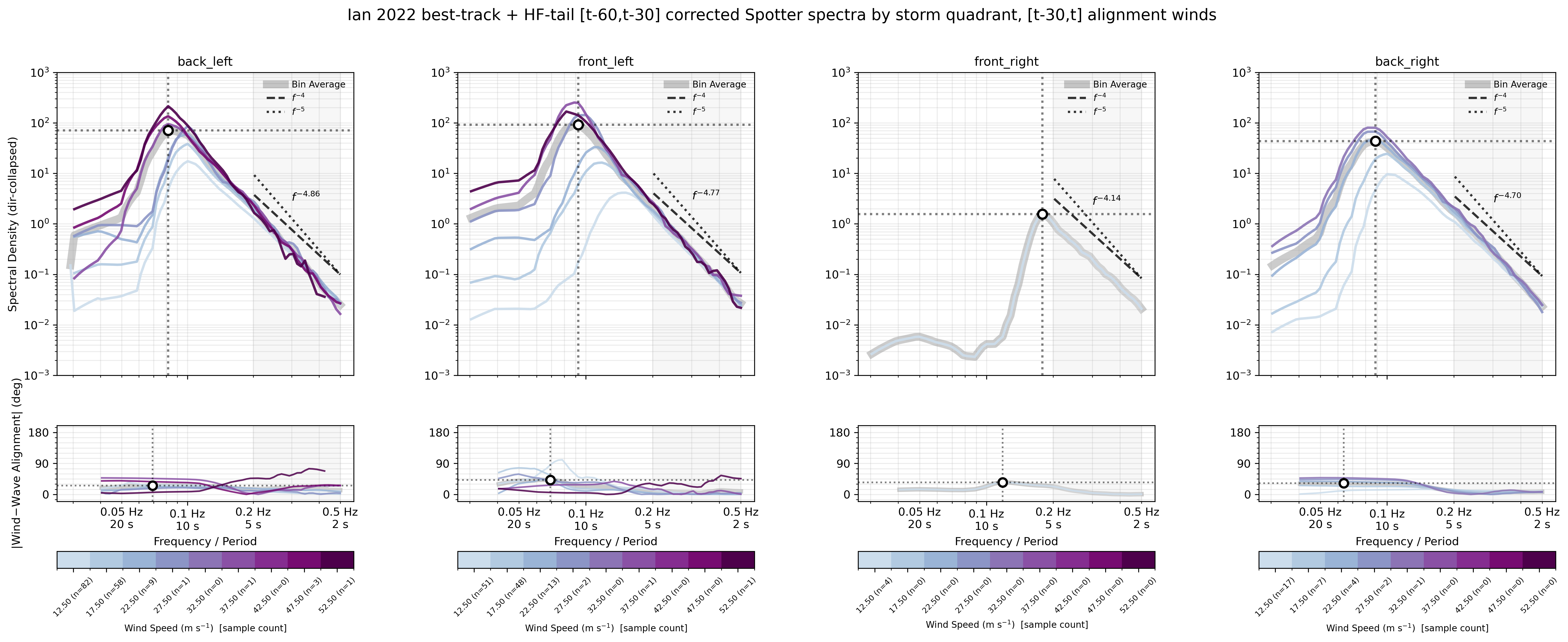
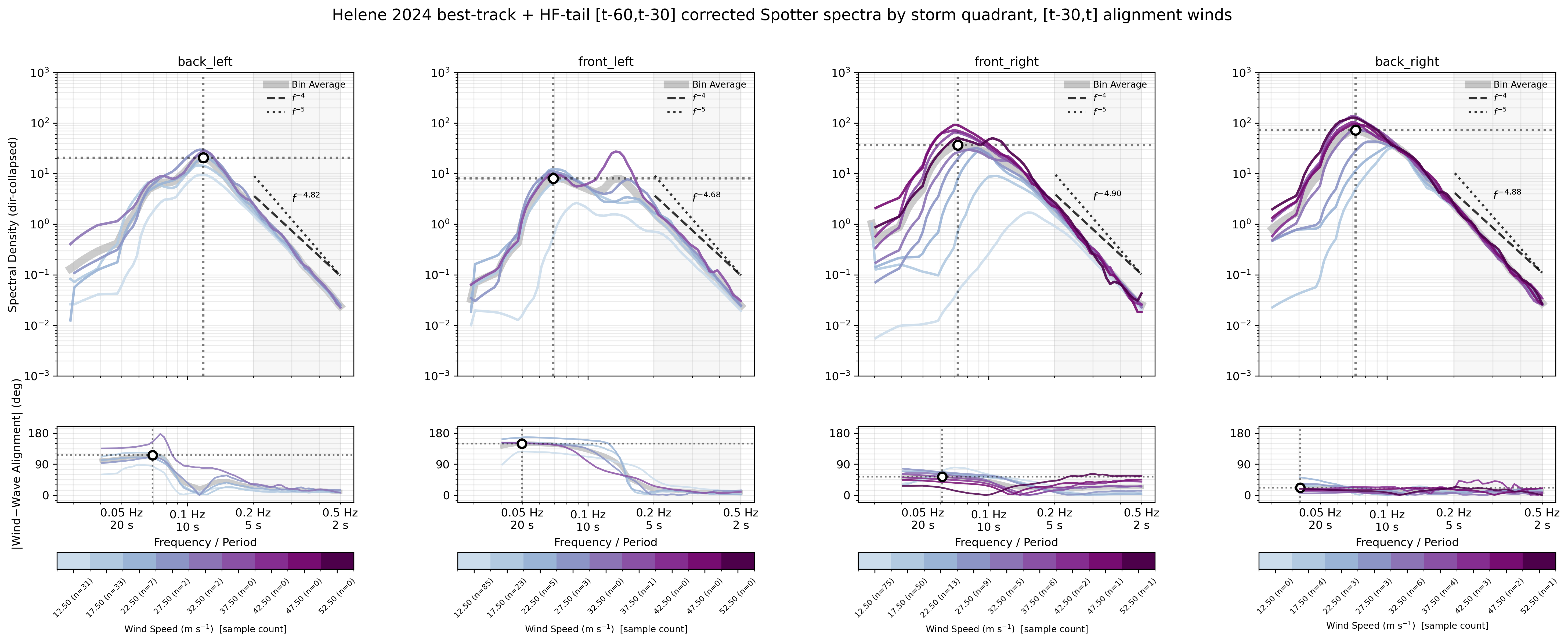
The corrected composites provide an internal validation of the adopted best-track plus HF-tail correction using the t-60 to t-30 min forcing interval. Across storms, the wind-speed bins generally form ordered spectral progressions, while the quadrant composites retain the expected spatial differences in spectral shape and wind–wave alignment. The consistency of these patterns across independent storms indicates that the correction produces stable storm-relative organization without artificially collapsing storm-to-storm variability.

The corrected composites provide an internal validation of the adopted best-track plus HF-tail correction using the t-60 to t-30 min forcing interval. Across storms, the wind-speed bins generally form ordered spectral progressions, while the quadrant composites retain the expected spatial differences in spectral shape and wind–wave alignment. The consistency of these patterns across independent storms indicates that the correction produces stable storm-relative organization without artificially collapsing storm-to-storm variability.

Aross storms, the right-side quadrants generally show stronger wind–wave alignment and more compact, energetic spectra, whereas the left-side quadrants retain larger low-frequency directional offsets and greater spectral complexity. These repeated contrasts are consistent with established TC-relative variations in effective fetch, wave age, and wave-field memory. Averaging the wind field over the same trailing 30-minute interval represented by each Spotter observation substantially improves the organization of the composites relative to using the instantaneous wind at the observation endpoint, reducing temporal mismatch between the forcing and measured spectrum.

Milton

Idalia

Ian

Helene

Discussion

Overall, the lead-time tests support the t-60 to t-30 min HF-tail correction as the most stable choice across storms. The correction primarily adjusts the along-track phase of the center and changes quadrant assignments near existing boundaries, rather than imposing a fundamentally different storm trajectory. The independent holdout experiment further supports this choice, showing that the selected 30-minute lead retains its improvement when evaluated on data excluded from the track-fitting procedure.

Using the corrected track together with winds averaged over the same 30-minute interval as the Spotter observations produces substantially cleaner quadrant composites. The recovered cross-quadrant differences are consistent across storms and align with established TC-relative variations in wave development and wind–wave alignment, supporting use of this framework for the subsequent normalized and history-dependent analyses.