Eulerian histories - wind only model

Framework

Overall goal

Given only the current wind and storm geometry, what wave state would we expect if the waves were in equilibrium with the local forcing?

In theory: $\text{Observed}=\text{Instantaneous baseline}+\text{History}+\text{Residual}$

The framework is applied separately to $H_s$, MSS, HFDS, $R_{hf}$, alignment, etc.

Method design

$H_s$ vs $\ln (H_s)$

Functional form selection

1. Linear regression

${\beta }_0+{\beta }_{1}U+{\beta }_2{U}^2$

Polynomial fits can be nonlinear in their estimated variable, while still using linear weights for the fit.

Using a polynomial fit generates one global equation, and under highly nonlinear conditions where the dataset can have a variety of functional forms at different stages. This results in artificial oscillation. While trying to improve the representation of one area, it becomes worse in another.

2. Splines

$f(U)={\sum }_i{\beta }_i{B}_i(U)$ → ${\beta }_1{B}_1+{\beta }_2{B}_2+{\beta }_3{B}_3+\cdots$

Where $B_i(U)$ are spline basis functions.

Instead of producing one equation, many small equations using a set of basis functions is combined to produce the final curve. This avoids the oscillation issue presented by polynomial fits.

3. GAMS

A generalized additive model uses individual splines for each predictor.

The generic $H_s={\beta }_0+{\beta }_{1}U+{\beta }_{2}R$ form becomes $H_s={\beta }_0+f_1(U)+f_2(R)$.

Where each $f_i$ is a spline.

The advantage of this approach is a combination of smooth independent variable curves, rather than optimized global functions, allowing each predictor to get the exact shape it needs.

Spline sensitivity & robustness framework

Goal

Determine whether the estimated smooth relationship between a predictor (e.g., wind speed) and a response (e.g., $H_s$) is:

• Statistically robust
• Physically interpretable
• Predictive on unseen storms
• Not an artifact of overfitting

Phase 1 - smoothness sensitivity

Vary the smoothing parameter

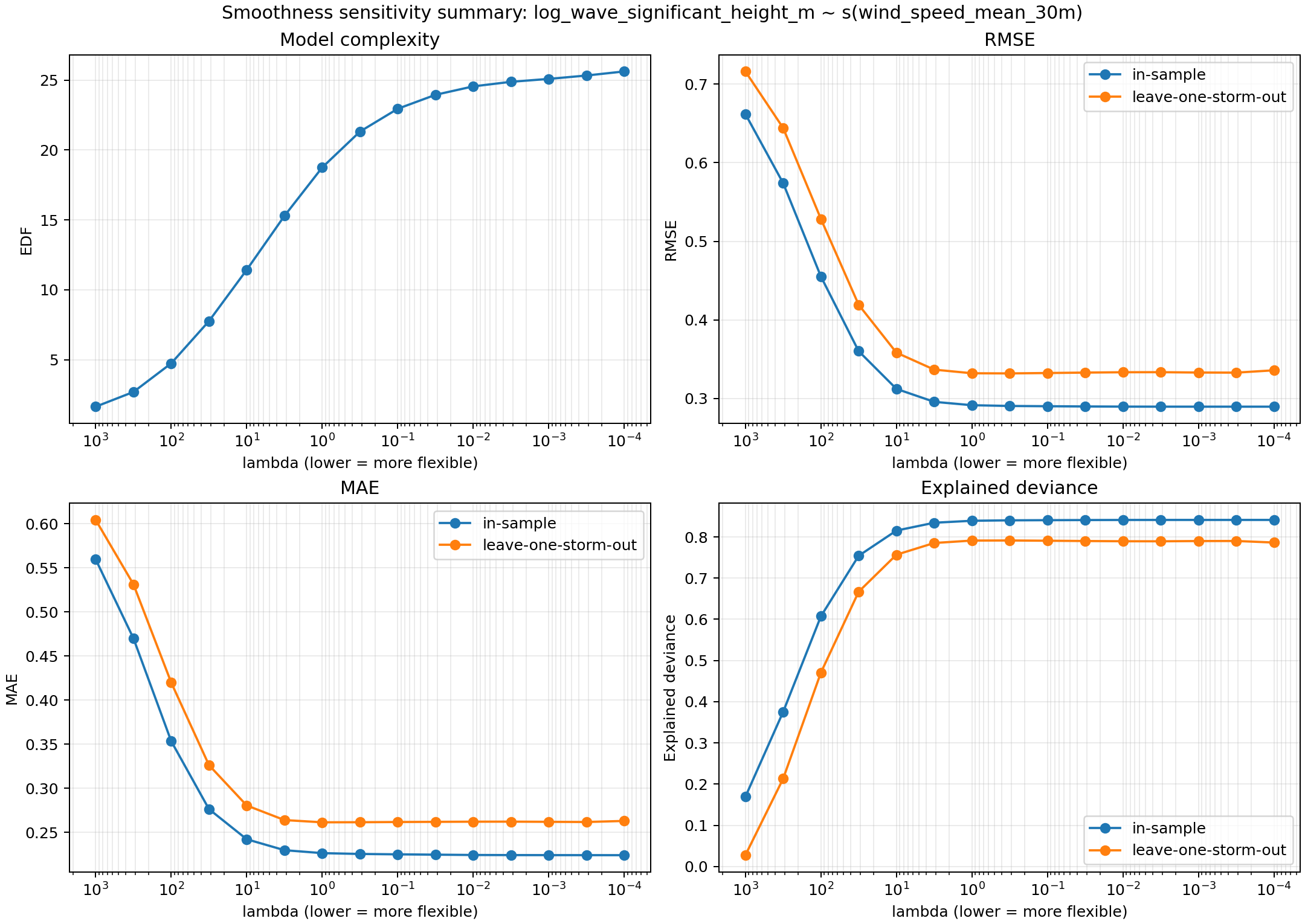
The first objective was to determine whether the shape of the wind-only generalized additive model (GAM) was primarily controlled by the smoothing penalty (λ), and to identify the range of smoothing that provides the best predictive performance without unnecessary model complexity.

The analysis was performed for both

• $H_s\sim s(U_{10})$
• $\log (H_s)\sim s(U_{10})$

using leave-one-storm-out cross-validation to evaluate generalization across storms.

For each value of λ, the following diagnostics were computed:

• Effective degrees of freedom (EDF)
• In-sample RMSE
• Leave-one-storm-out RMSE
• In-sample MAE
• Leave-one-storm-out MAE
• Explained deviance
• The fitted spline shape

The smoothing penalty was varied over several orders of magnitude, from very stiff fits (large λ) to highly flexible fits (small λ).

Results

As expected, decreasing λ increased the effective degrees of freedom, allowing progressively more flexible spline shapes. The EDF increased smoothly from approximately 2 to approximately 25 across the tested λ range.

Model skill improved rapidly as λ decreased from very large values, but all performance metrics reached a broad plateau once λ was approximately between 1 and 10. Beyond this point:

• leave-one-storm-out RMSE changed very little,
• leave-one-storm-out MAE remained nearly constant,
• explained deviance no longer increased appreciably.

Further reductions in λ increased spline complexity but produced essentially no improvement in predictive performance.

This behavior was nearly identical for both the linear and log-transformed response variables, indicating that the optimal amount of smoothing is relatively insensitive to the response transformation.

Spline Behavior

Overlaying the fitted splines revealed two important behaviors.

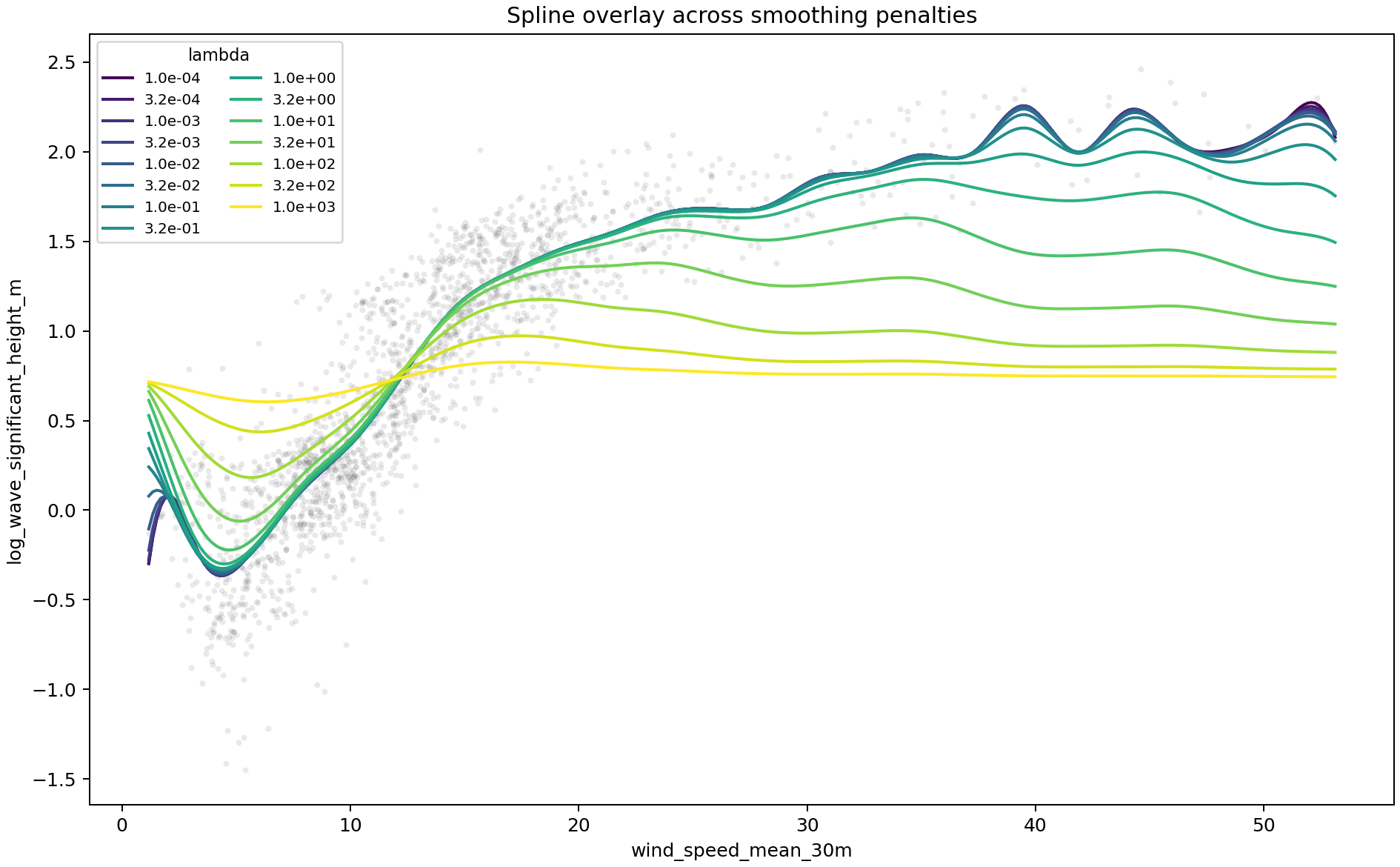
First, overly large λ values produced underfit models that failed to capture the nonlinear increase of wave height with wind speed.

Second, once λ became sufficiently small, all spline solutions converged toward nearly the same shape. Although these more flexible splines contained oscillatory structure at high wind speeds, the oscillations persisted over a wide range of λ values rather than appearing only for extremely flexible fits.

This indicates that the remaining curvature is not primarily controlled by the smoothing penalty.

Interpretation

The sensitivity analysis demonstrates that λ is not the limiting factor controlling model quality.

Instead:

• predictive performance becomes essentially insensitive to λ once moderate flexibility is reached,
• increasing flexibility beyond this point only increases model complexity,
• persistent oscillations in the fitted relationship likely arise from other aspects of the model, including the spline basis, basis dimension, sparse sampling at high wind speeds, or physical variability that cannot be represented by a one-dimensional wind-only relationship.

The log-transformed response provides a more homogeneous variance structure and will therefore be adopted for subsequent model development.

Conclusions

The λ sensitivity study reached several conclusions:

• A broad optimum exists near λ ≈ 1–10.
• Additional reductions in λ provide negligible improvements in predictive skill.
• The remaining spline oscillations are not caused by the smoothing penalty alone.
• The logarithmic response variable is preferred because it better stabilizes variance while maintaining essentially identical predictive performance.
• Future work should focus on spline basis selection, basis dimension, and ultimately the inclusion of additional physically meaningful predictors rather than further optimization of λ.

Phase 2 - Spline basis selection

Following the smoothing-parameter sensitivity analysis, the next step was to determine whether the remaining structure in the wind-only model depended on the choice of spline basis or basis dimension. Three spline families were evaluated (thin-plate regression splines, cubic regression splines, and P-splines), together with their corresponding shrinkage variants, over a range of basis dimensions (k=6–30) using leave-one-storm-out cross-validation.

A spline can be thought of as a flexible ruler that bends to follow the overall relationship between wind speed and wave height. Different spline bases differ in how they are allowed to bend, but all attempt to balance fitting the observations against remaining smooth. The shrinkage variants introduce an additional penalty that discourages the model from retaining weak or unsupported features. In practice, this allows the spline to ignore unnecessary complexity rather than preserving subtle curvature simply because it is mathematically possible.

Among the tested models, a thin-plate shrinkage spline with k=8 was selected as the provisional wind-only baseline. Although the one-standard-error rule initially favored the simpler k=6 thin-plate shrinkage spline, the k=8 model had effectively indistinguishable cross-validated RMSE, MAE, and explained deviance, while requiring only a modest increase in effective degrees of freedom. A cubic regression spline with k=10 produced the lowest raw cross-validation error, but the improvement was small relative to its greater complexity. The k=8 thin-plate shrinkage model was therefore retained because it preserved the same relationship over the well-sampled wind range while producing a more conservative and physically plausible upper-boundary shape than the k=6 fit.

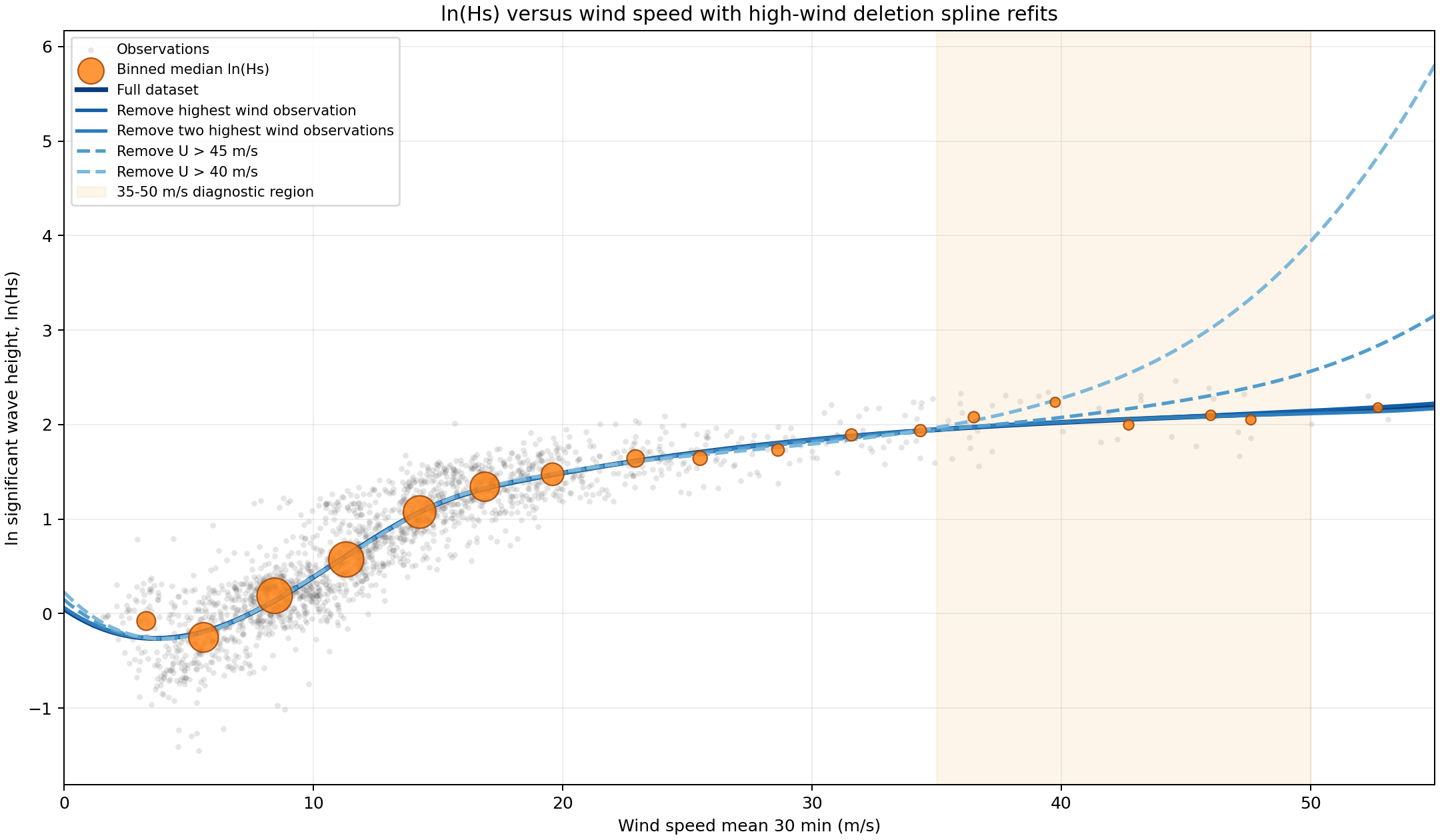
The candidate spline fits agreed closely over the wind-speed range containing most observations, approximately 8–35 m s${}^{-1}$. Differences between spline families occurred primarily at very low wind speeds and above approximately 35–40 m s${}^{-1}$, where observational support becomes sparse and leverage increases. High-wind influence testing showed that the selected k=8 fit was insensitive to removing any individual high-wind observation and to removing the one or two highest-wind observations; the refitted curves remained nearly identical and the estimated high-wind slope remained positive. However, removing all observations above 40 or 45 m s${}^{-1}$ produced unstable extrapolation beyond the revised data range. These results indicate that the broad wind–wave relationship is robust within the observed range, while the exact endpoint behavior remains data-limited and should not be interpreted as a well-constrained physical growth law.

Metrics

Effective Degrees of Freedom (EDF)

The complexity of each fitted spline is quantified by its effective degrees of freedom (EDF). Unlike the basis dimension k, which specifies the maximum complexity available to the spline, the EDF measures how much of that flexibility is actually used after penalization.

Mathematically, the EDF is defined as

$\mathrm{EDF}=\mathrm{trace}(\mathbf{H})$,

where $\mathbf{H}$ is the smoothing matrix that maps the observed responses to the fitted values,

$\hat{\mathbf{y}}=\mathbf{Hy}$.

An EDF close to one corresponds to a nearly linear relationship, while larger values indicate increasingly nonlinear behavior. The selected model has an EDF of approximately six, indicating that the relationship is moderately nonlinear without exhibiting unnecessary complexity.

Root Mean Square Error (RMSE)

Model accuracy was evaluated using the root mean square error,

$\mathrm{RMSE}=\sqrt{\frac{1}{n}{\sum }_{i=1}^n{\left(y_i-{\hat{y}}_i\right)}^2}$,

where $y_i$ is the observed value and ${\hat{y}}_i$ is the model prediction.

Because the residuals are squared before averaging, RMSE gives greater weight to large prediction errors. It therefore measures how well the model avoids substantial mistakes and is particularly sensitive to poorly predicted observations.

Mean Absolute Error (MAE)

The mean absolute error is defined as

$\mathrm{MAE}=\frac{1}{n}{\sum }_{i=1}^n\left|y_i-{\hat{y}}_i\right|$.

Unlike RMSE, every residual contributes proportionally to the average error. MAE therefore measures the typical prediction error and is less sensitive to occasional large residuals. Comparing MAE and RMSE provides insight into whether model performance is dominated by a few poorly predicted observations or by more uniform prediction errors across the dataset.

Phase 3 - Leave one storm out cross validation (LOOSO)

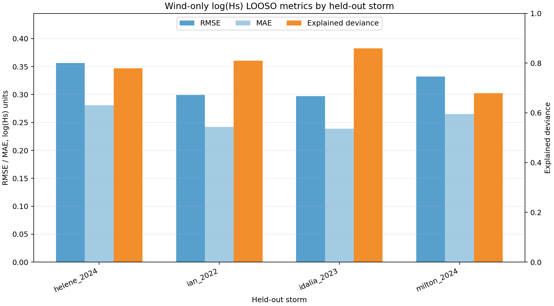
To evaluate how well the wind-only baseline generalizes across independent storms, model performance was assessed using leave-one-storm-out cross-validation (LOOSO). In each iteration, the spline model was trained using observations from three storms and then evaluated on the remaining storm, repeating the procedure until each storm had served once as the independent test dataset. Unlike conventional random cross-validation, LOOSO prevents observations from the same storm appearing in both the training and testing sets, providing a more rigorous assessment of the model’s ability to capture a general wind–wave relationship rather than storm-specific characteristics.

Model performance was quantified using the root mean squared error (RMSE), mean absolute error (MAE), and explained deviance for each held-out storm. Similar predictive skill across all four folds indicates that the fitted relationship is stable and transferable between storms, whereas substantial degradation for an individual storm would suggest overfitting or dependence on storm-specific behavior. The relatively consistent performance obtained across the four tropical cyclones demonstrates that the instantaneous wind-only baseline captures a robust first-order relationship between wind speed and significant wave height, providing an appropriate reference model for evaluating the additional explanatory value of storm structure and forcing-history predictors.

Residuals

Diagnostic pannel description

1. Residuals vs fitted : is the mean relationship removed?
2. Residuals vs wind : is wind speed still missing from the model?
3. Absolute residuals : is variance constant?
4. Q-Q plot : Are residuals approximately gaussian?
5. Residuals by storm : does the model generalize?
6. Residual vs radius : is radius still important?
7. Residual by quadrant : does storm geometry matter?
8. Observed vs predicted : overall fit quality?

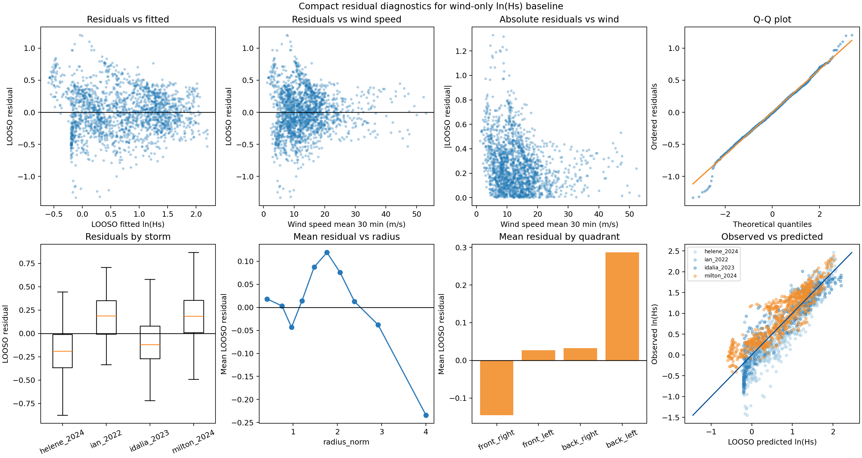
**$H_s$ interpretation

• The wind-only GAM has successfully captured the dominant relationship between wind speed and significant wave height.
• The residuals behave well statistically: they are centered near zero, approximately Gaussian, and show no remaining dependence on wind speed.
• The remaining systematic residual structure is organized by storm-relative radius and quadrant rather than by wind speed itself, indicating that these variables contain additional physical information beyond instantaneous wind forcing.

Model evaluation

Applying the model fitting pipeline to other predictors.

Intrinsic MSS

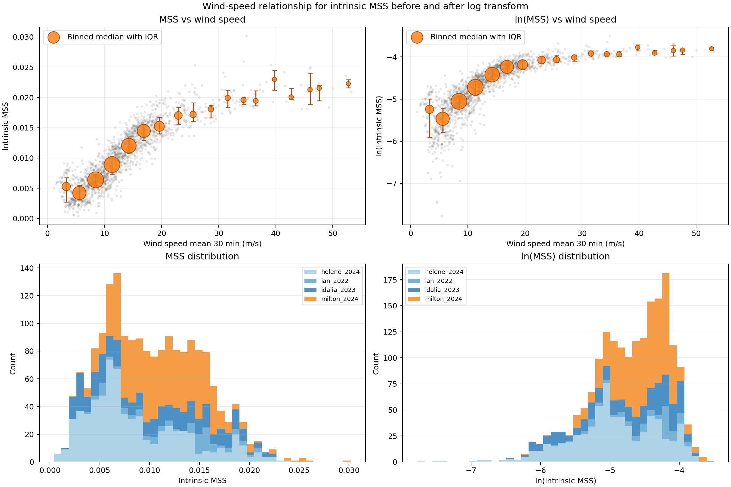
The intrinsic mean square slope analysis began by comparing the response on its original and logarithmic scales. Unlike significant wave height, intrinsic MSS did not show a strong variance increase or severe positive skew on the raw scale. The raw distribution was only moderately asymmetric, while the logarithmic transformation stretched the lowest MSS values and produced a more strongly skewed lower tail. The wind-speed relationships retained the same broad shape under both formulations, but the log transformation did not provide an obvious improvement in symmetry or variance stabilization. This suggested that intrinsic MSS could reasonably be modeled on its original scale.

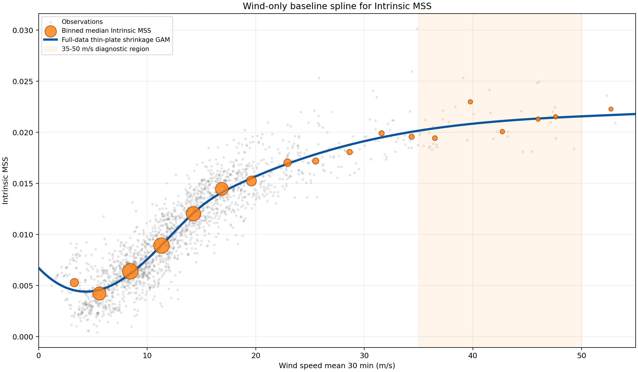
The selected wind-only thin-plate shrinkage GAM captures a clear nonlinear relationship between wind speed and intrinsic MSS. MSS is lowest at weak winds, increases rapidly through approximately 7–20 m s${}^{-1}$, and then transitions into progressively slower growth above roughly 20–30 m s${}^{-1}$. At the highest observed wind speeds, the fitted relationship approaches a broad plateau near MSS values of approximately 0.02. The spline closely follows the binned medians across the well-sampled part of the wind range. Observational support becomes much weaker above approximately 35 m s${}^{-1}$, so the exact high-wind slope should be interpreted cautiously, although the fitted curve remains smooth and physically plausible.

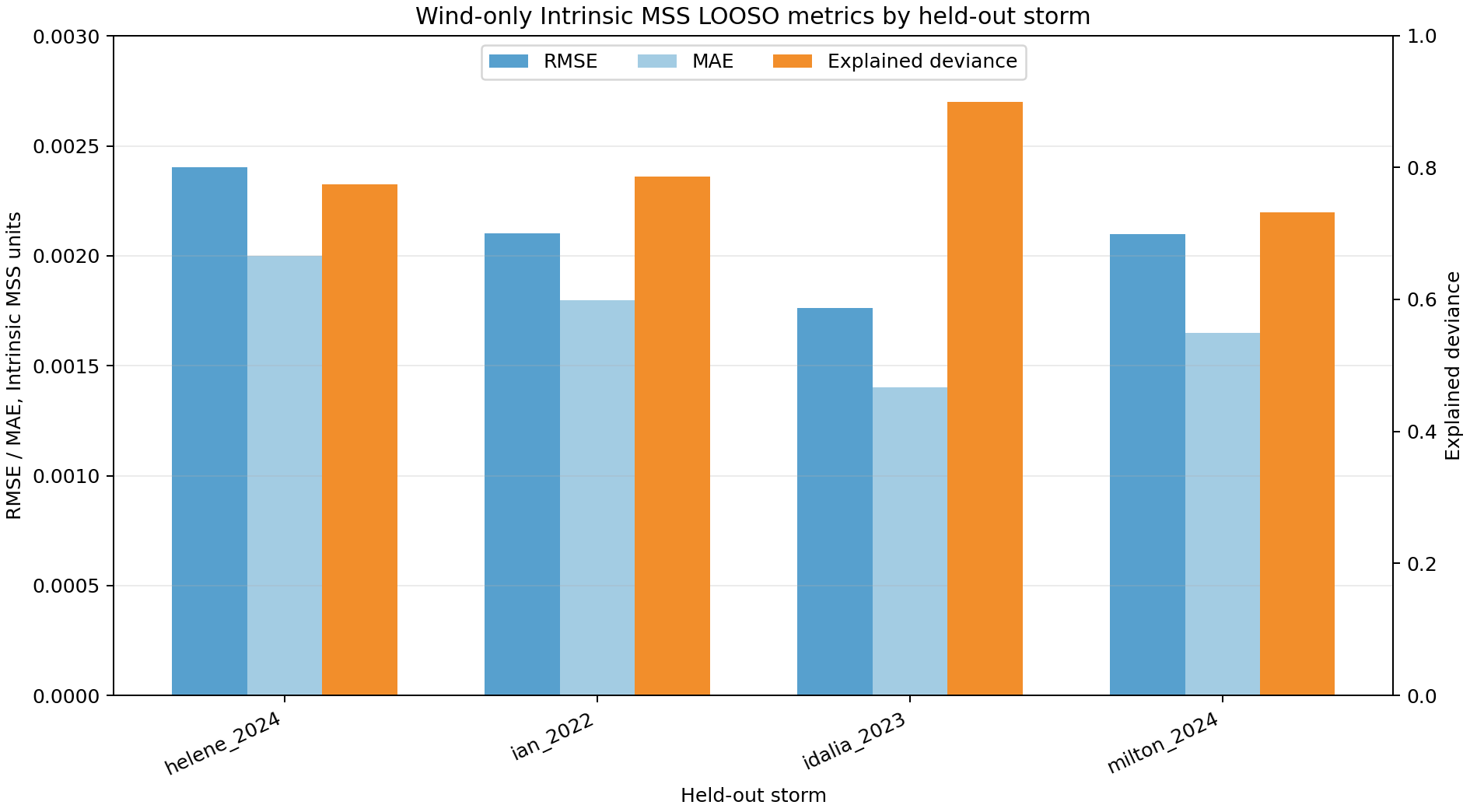
Leave-one-storm-out validation shows that this relationship generalizes well across all four storms. When each storm is excluded in turn and predicted using a model trained on the other three, explained deviance remains high, ranging from approximately 0.73 for Milton to about 0.90 for Idalia. RMSE and MAE also remain relatively consistent among storms, with no catastrophic loss of skill for any held-out case. These results indicate that the fitted MSS–wind relationship is not simply reproducing storm-specific patterns; it represents a robust first-order relationship that transfers reasonably well to storms not included in model fitting.

The residual diagnostics further support retaining MSS on its original scale. Residuals remain broadly centered around zero across fitted values and wind speeds, with no strong remaining mean dependence on wind speed. The Q–Q plot follows the Gaussian reference closely through most of the distribution, with only a small upper-tail departure caused by a few unusually large positive residuals. The residual spread remains somewhat greater at low and moderate wind speeds, but the variance pattern is substantially better behaved than for the logarithmic formulation.

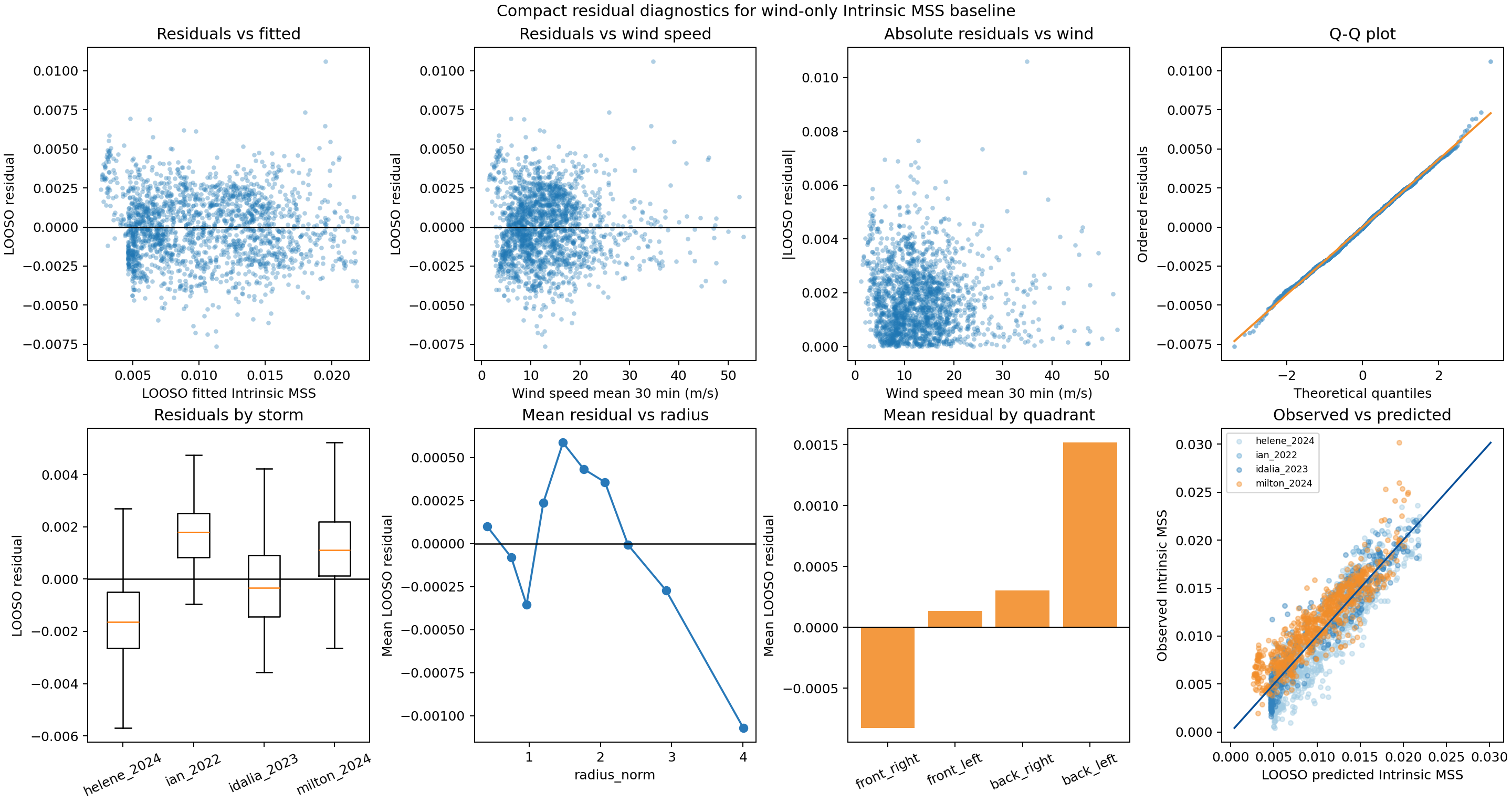
Systematic storm-to-storm differences remain after removing the wind-speed relationship. Helene and Idalia tend to have negative residuals, meaning the wind-only model generally predicts larger MSS than observed, while Ian and Milton tend to have positive residuals. These offsets are moderate and are consistent with the idea that storm size, geometry, translation, and forcing history modify MSS beyond the effect of instantaneous wind speed.

The residuals also retain coherent storm-relative structure. Mean residuals vary nonlinearly with normalized radius, becoming positive around normalized radii of approximately 1.3–2 before declining and becoming negative farther from the storm center. Quadrant differences are also evident: the front-right quadrant has negative residuals, while the back-left quadrant has the largest positive residuals. These patterns show that instantaneous wind speed explains most of the MSS variability, but not all of it. Radius and storm-relative geometry contain additional physical information that should be evaluated in the next modeling stage.

Overall, the raw intrinsic MSS model provides the stronger baseline. It preserves direct physical interpretability, produces better-behaved residuals, and generalizes consistently across storms. The main conclusion is that wind speed controls the dominant nonlinear increase and high-wind saturation of intrinsic MSS, while the remaining variability is systematically organized by storm identity, normalized radius, and quadrant.

High frequency energy fraction

After inverse-transforming predictions to the original $R_{hf}$ scale, differences in leave-one-storm-out prediction skill among the raw, logarithmic, and logit formulations were small and varied by storm. The logit model performed best for Ian and Idalia, the logarithmic model performed best for Milton, and the raw model was competitive for Helene. Because no transformation uniformly minimized original-scale error, the final choice was based jointly on predictive performance and residual behavior. The logarithmic model was retained as the primary baseline because it provided the most stable conditional residual distribution without the strong boundary amplification seen under the logit transformation. The logit model was retained as a sensitivity check.

Peak frequency

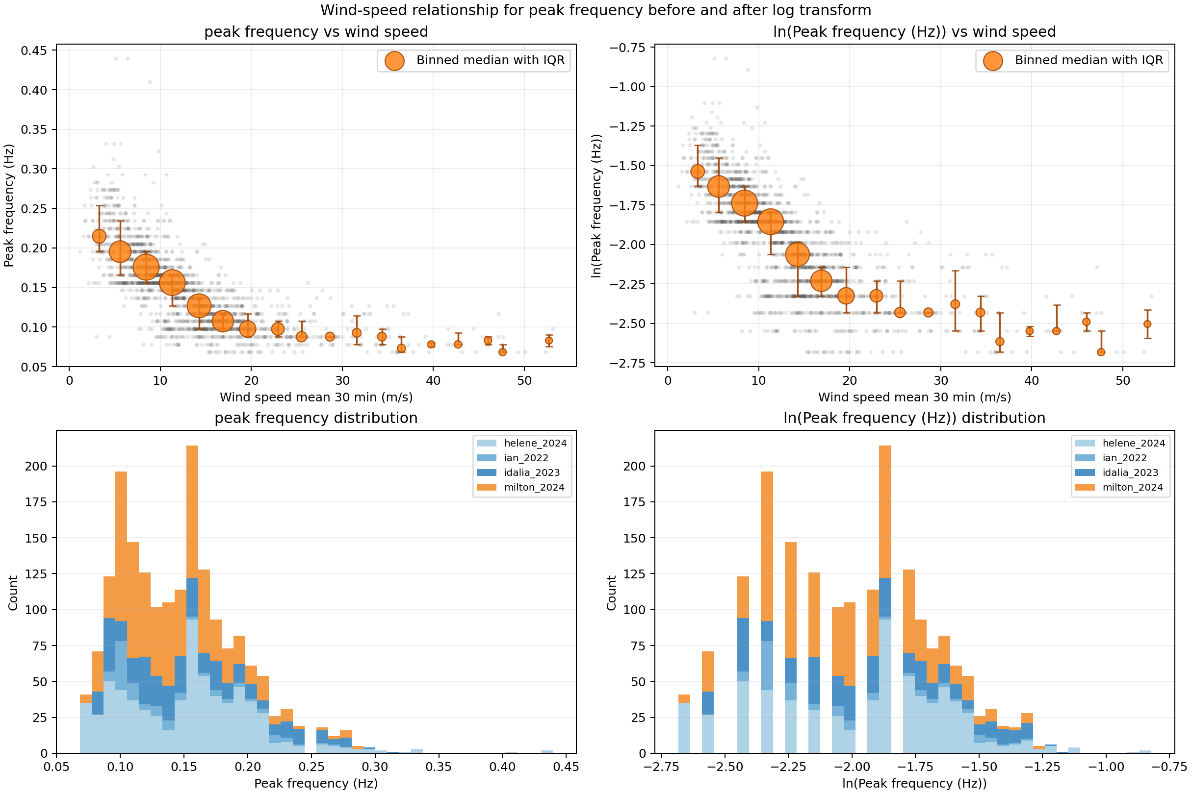
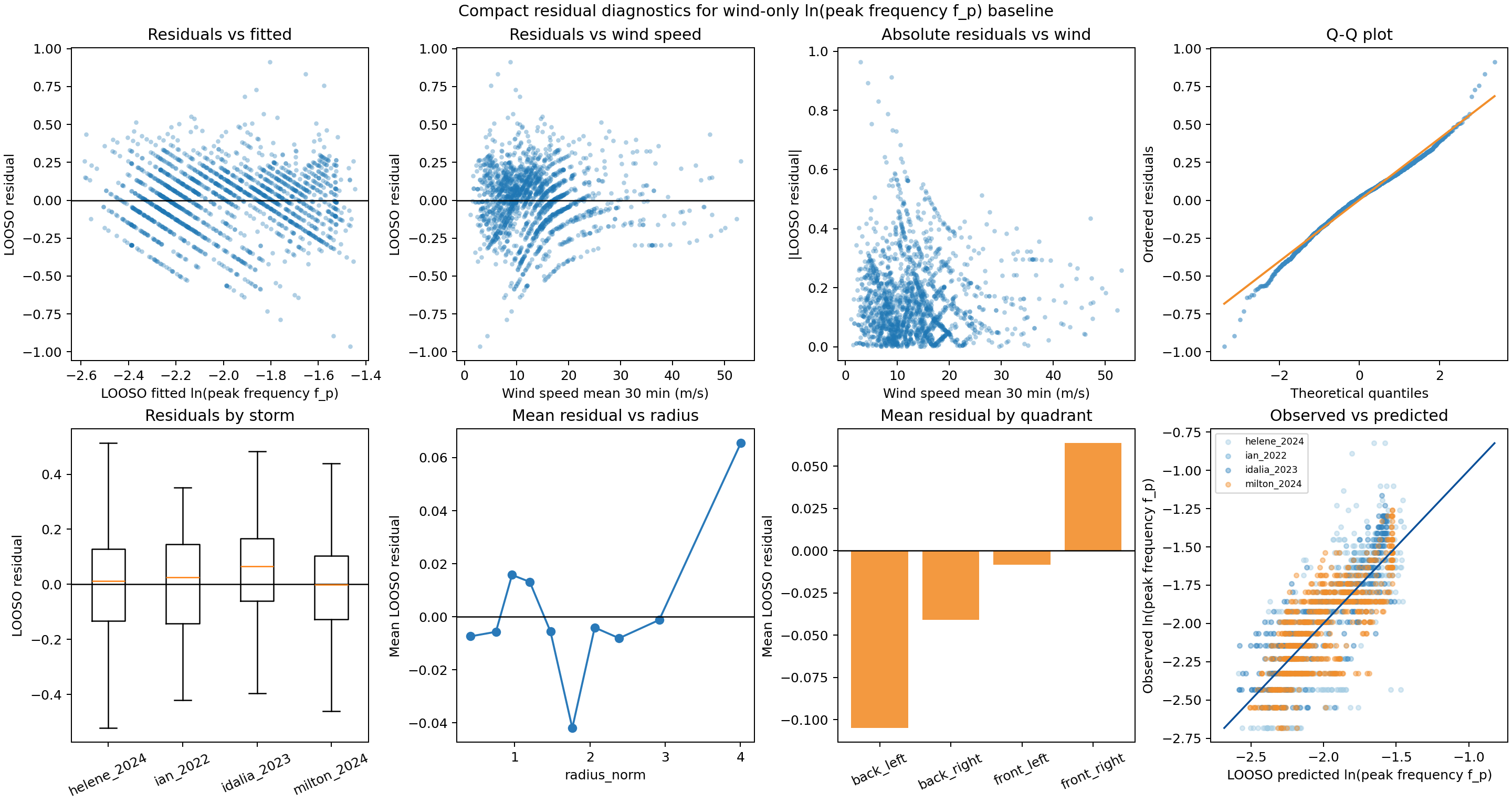
The relationship between peak frequency and wind speed is strongly nonlinear, with the majority of the evolution occurring at relatively modest wind speeds before gradually approaching an asymptotic state as the storm intensifies. Because peak frequency is strictly positive and exhibits increasing skew toward lower wind speeds, both the raw and logarithmically transformed variables were examined to determine which representation provided the most appropriate statistical framework. The logarithmic transformation modestly reduced distributional skewness while preserving the underlying physical relationship between wind speed and peak frequency. Although the improvement was less dramatic than for intrinsic MSS, residual diagnostics exhibited a more nearly Gaussian distribution and comparable predictive performance, motivating the use of the logarithmic formulation for the wind-only baseline.

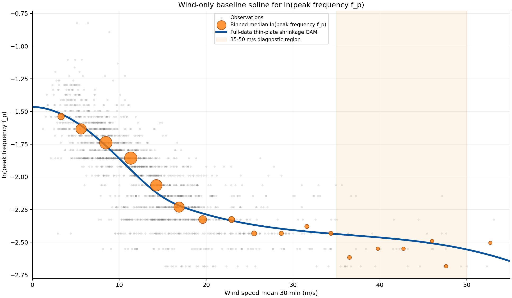
A thin-plate shrinkage GAM was then fit to the transformed observations to estimate the first-order dependence of peak frequency on local wind speed. The resulting smooth reproduces the rapid decrease in peak frequency during early wave growth before transitioning to a much weaker dependence above approximately 20 m s${}^{-1}$. At the highest wind speeds, where observations become increasingly sparse, the penalized spline remains well behaved and follows the central tendency of the available observations without introducing unrealistic oscillations. This behavior indicates that the fitted relationship captures the dominant wind-speed dependence while remaining appropriately regularized in regions of limited observational support.

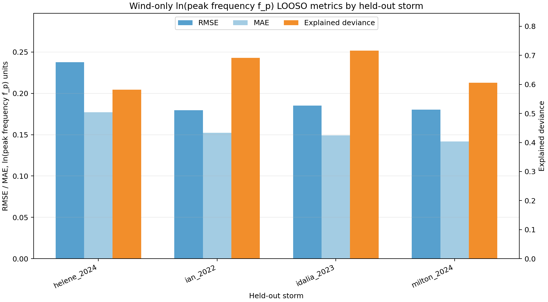
The generality of this baseline was evaluated using leave-one-storm-out cross validation, in which each storm was withheld during fitting and used exclusively for prediction. Predictive skill remained consistent across the independent storms, indicating that the fitted relationship is not simply reproducing storm-specific characteristics but instead represents a transferable wind-speed dependence common to multiple tropical cyclones. This provides confidence that the spline can serve as a robust first-order baseline against which additional physical controls may be evaluated.

Finally, residual diagnostics were examined to determine whether systematic structure remained after removing the wind-speed dependence. Residuals were centered near zero across fitted values and wind speed, indicating that the baseline successfully captured the dominant trend. However, coherent residual patterns persisted with normalized radius and storm-relative quadrant, suggesting that local wind speed alone is insufficient to fully describe the observed variability. The persistence of these organized residuals motivates the introduction of additional predictors describing storm geometry and forcing history, which are investigated in the following sections.

High frequency directional spread

HF directional spread should be modeled on the logarithmic scale because the transformation substantially reduces right skew, stabilizes the variance, and prevents a small number of very broad directional distributions from dominating the fit.

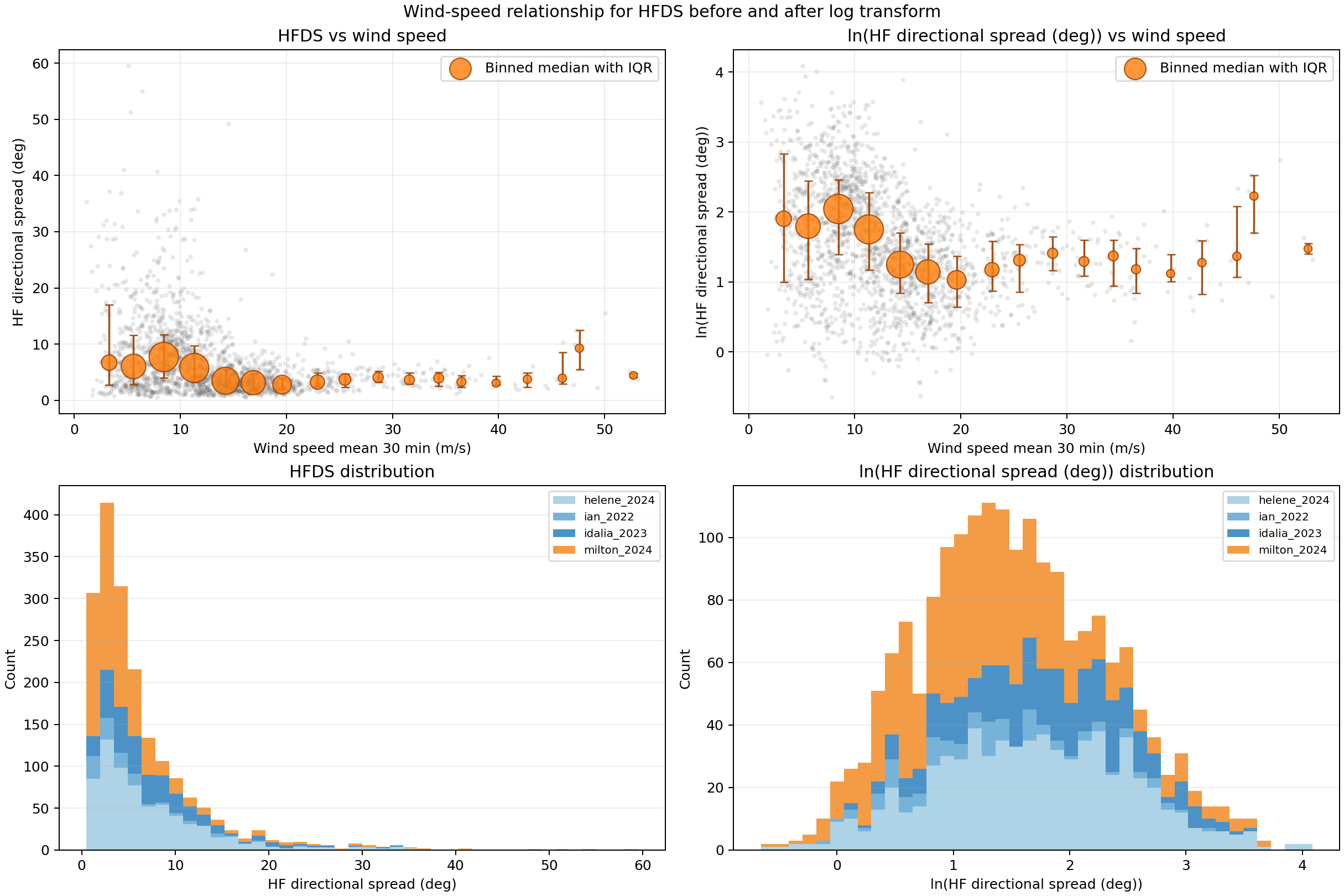
Unlike the previous variables, transforming HF directional spread primarily improved the statistical properties of the response rather than the predictive skill of the wind-only baseline. Applying a logarithmic transformation substantially reduced the strong right-skew present in the raw observations and produced residuals that more closely satisfied the assumptions of the Gaussian GAM framework. However, this statistical improvement did not translate into a substantially more descriptive wind-speed relationship. Although the transformed baseline captures the broad tendency for HF directional spread to decrease from weak to moderate winds before leveling off, the explained deviance remains low and varies considerably between storms, with several held-out cases exhibiting little or no predictive skill beyond a climatological mean.

Examination of the residual diagnostics further indicates that a large fraction of the remaining variability is organized rather than random. Systematic differences persist between storms, storm-relative quadrants, and normalized radius despite accounting for the instantaneous wind-speed dependence. This suggests that HF directional spread is fundamentally less controlled by the instantaneous local wind forcing than variables such as significant wave height, peak frequency, or high-frequency energy fraction. Instead, much of its variability likely reflects the integrated evolution of the wave field, including directional wave history, storm-relative geometry, and the alignment between the existing wave spectrum and the evolving wind field. Consequently, while the logarithmic transformation is retained because it provides a statistically appropriate response variable, the limited performance of the wind-only baseline indicates that HF directional spread should be viewed as a higher-order descriptor whose dominant controls lie beyond instantaneous wind speed.

The first stage of the analysis identifies variables that are largely determined by instantaneous forcing, establishing a physically meaningful baseline. The remaining unexplained variability is not random but concentrated within descriptors of wave organization, particularly peak directional spread and high-frequency directional spread. Because these variables cannot be reproduced from local wind speed alone, they emerge as natural candidates for the history-dependent degrees of freedom in the wave-state continuum. Rather than representing noise, they likely encode the integrated effects of storm-relative evolution, wave propagation, and forcing history, providing a clear motivation for introducing lagged wind histories and history-based normalization in the next stage of the analysis.